


欢迎大家关注全网生信学习者系列:
- WX公zhong号:生信学习者
- Xiao hong书:生信学习者
- 知hu:生信学习者
- CDSN:生信学习者2
介绍
本教程用于对研究的数据汇总和数据探索,其中用于可视化的图形有柱状图、森林图等。
森林图是一种常用于展示多个研究结果的统计图表。它显示了各个研究的效应量(effect size)或优势比(odds ratio, OR)以及它们的95%置信区间(confidence interval, CI)。通过森林图,研究者可以快速地比较和评估不同变量对结局变量的影响。
-
OR(Odds Ratio):优势比,用于表示某个因素与结果之间的关联强度。OR值大于1表示该因素增加结果发生的可能性,OR值小于1表示该因素减少结果发生的可能性。OR值等于1则表示没有影响。
-
95% CI(95% Confidence Interval):95%置信区间,表示我们有95%的把握认为真实的效应量位于这个区间内。如果置信区间不包含1,则通常认为该效应是统计学上显著的。
-
P值:用来测试统计假设,即观察到的效应是否可能仅仅是随机发生的。P值小于0.05通常被认为是统计学上显著的。
加载R包
#| warning: false
#| message: false

library(tidyverse)
library(readr)
library(magrittr)
library(qwraps2)
library(ggpubr)
library(ggsci)
library(CLME)
导入数据
大家通过以下链接下载数据:
- 百度网盘链接:https://pan.baidu.com/s/1fz5tWy4mpJ7nd6C260abtg
- 提取码: 请关注WX公zhong号_生信学习者_后台发送 复现gmsb 获取提取码
df_merge <- read_csv("./data/GMSB-data/df_merge.csv", show_col_types = FALSE)
df_seq <- read_csv("./data/GMSB-data/per-sample-fastq-counts.csv", show_col_types = FALSE)
数据预处理
df_v1 <- df_merge %>%
  dplyr::filter(visit == "v1")

df_seq <- df_seq %>%
  dplyr::filter(`Sample ID` %in% df_v1$sampleid)
测序通量
评估二代测序的测序通量,在后续校正测序通量对检验结果的影响
tol_reads <- sum(df_seq$`Sequence count`)
mean_reads <- mean(df_seq$`Sequence count`)
med_reads <- median(df_seq$`Sequence count`)

bin_length <- 4000
b <- seq(0, 140000, bin_length)

p <- df_seq %>%
  ggplot(aes(x = `Sequence count`)) +
  geom_histogram(aes(y = ..count..), breaks = b, color = "black", fill = "lightblue1") +
  geom_density(aes(y = ..density..* (nrow(df_seq) * bin_length)), color = "brown3") +
  scale_x_continuous(breaks = seq(20000, 140000, 40000)) +
  labs(x = "Read Number", y = "Number of Samples", title = "Reads per sample",
       subtitle = paste0("Min = ", min(df_seq$`Sequence count`), " (",
                         df_seq$`Sample ID`[which.min(df_seq$`Sequence count`)], ") \n",
                         "Max = ", max(df_seq$`Sequence count`), " (",
                         df_seq$`Sample ID`[which.max(df_seq$`Sequence count`)], ")")) +
  theme_bw() +
  theme(plot.title = element_text(hjust = 0.5),
        plot.subtitle = element_text(hjust = 0.5))
p
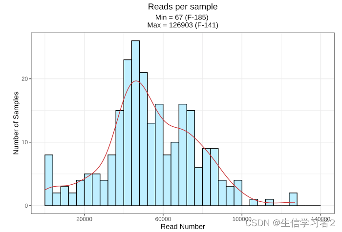
结果:测序通量
-
Number of samples:
r nrow(df_seq) -
Total number of sequences:
r tol_reads -
Average reads:
r mean_reads -
Median reads:
r med_reads
分组数据分布
不同分组的结局变量status(seroconverter (SC) rates 和 seronegative control (NC))与其他变量的相关性分析
Primary group: 按照频率分组1
-
G1: # receptive anal intercourse = 0
-
G2: # receptive anal intercourse = 1
-
G3: # receptive anal intercourse = 2 - 5
-
G4: # receptive anal intercourse = 6 +
Secondary group: 按照频率分组2
-
G1: # receptive anal intercourse = 0
-
G2: # receptive anal intercourse = 1
-
G3: # receptive anal intercourse = 2 - 3
-
G4: # receptive anal intercourse = 4 - 8
-
G5: # receptive anal intercourse = 9 +
recept_anal <- df_v1$recept_anal
recept_anal <- recept_anal[!is.na(recept_anal)]

print(paste0("mean = ", round(mean(recept_anal)),
             ", median = ", median(recept_anal),
             ", min = ", min(recept_anal),
             ", max = ", max(recept_anal)))

p_expose <- df_v1 %>%
  ggplot(aes(x = recept_anal)) +
  geom_histogram(aes(y = ..count..), bins = 100, color = "black", fill = "lightblue1") +
  labs(x = "Number of Receptive Anal Intercourse", y = "Frequency") +
  theme_bw() +
  theme(plot.title = element_text(hjust = 0.5),
        plot.subtitle = element_text(hjust = 0.5))

p_expose
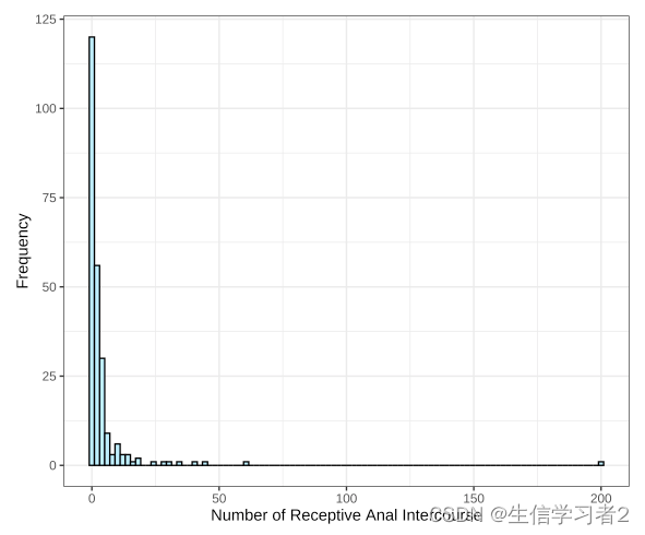
结果:数据分布呈现偏态分布,大部分人集中在0-10之间。
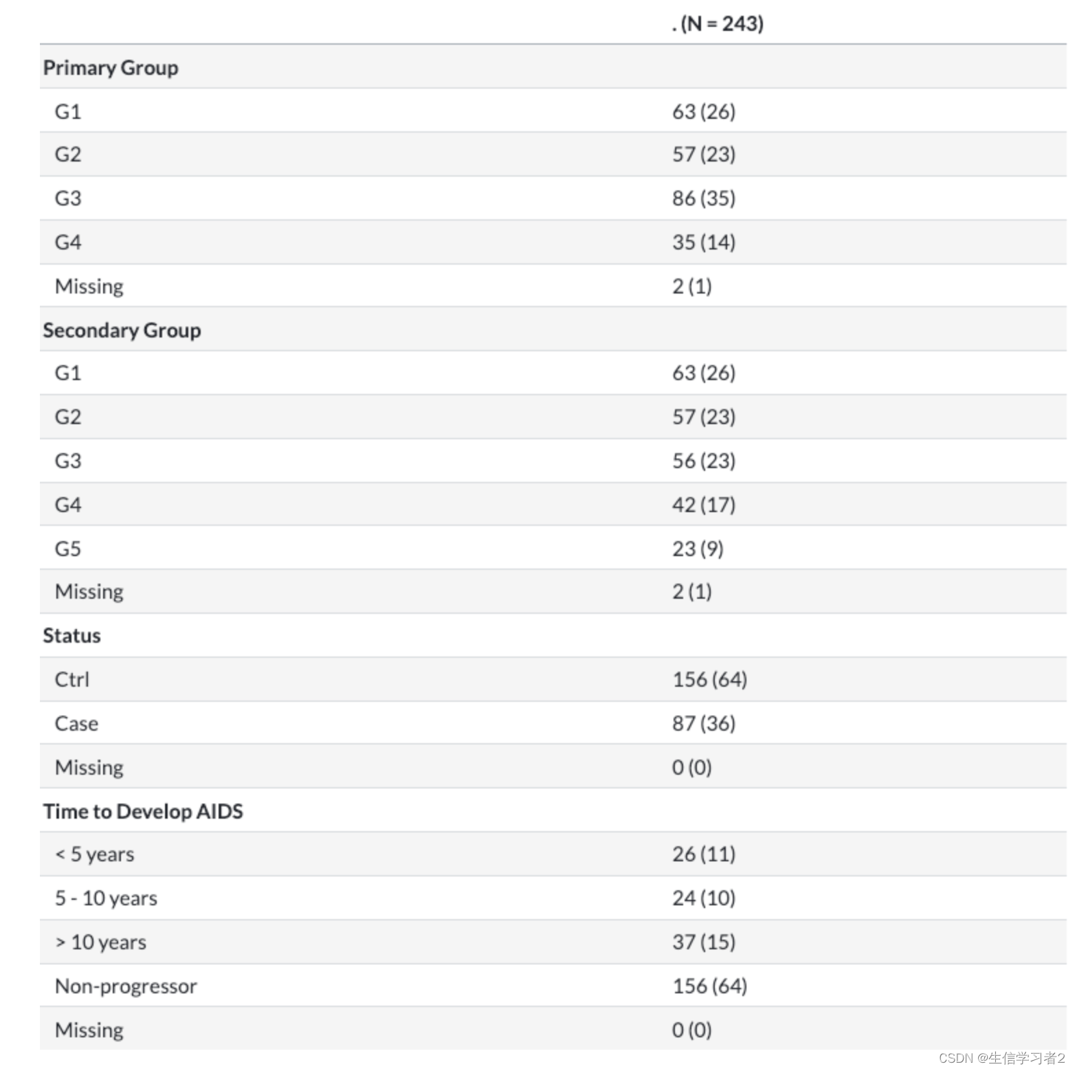
数据汇总表格
options(qwraps2_markup = "markdown") # markdown

summary_template <-
  list("Primary Group" =
         list("G1" = ~ n_perc0(group1 == "g1", na_rm = T),
              "G2" = ~ n_perc0(group1 == "g2", na_rm = T),
              "G3" = ~ n_perc0(group1 == "g3", na_rm = T),
              "G4" = ~ n_perc0(group1 == "g4", na_rm = T),
              "Missing" = ~ n_perc0(group1 == "missing", na_rm = T)),
       "Secondary Group" =
         list("G1" = ~ n_perc0(group2 == "g1", na_rm = T),
              "G2" = ~ n_perc0(group2 == "g2", na_rm = T),
              "G3" = ~ n_perc0(group2 == "g3", na_rm = T),
              "G4" = ~ n_perc0(group2 == "g4", na_rm = T),
              "G5" = ~ n_perc0(group2 == "g5", na_rm = T),
              "Missing" = ~ n_perc0(group2 == "missing", na_rm = T)),
       "Status" =
         list("Ctrl" = ~ n_perc0(status == "nc", na_rm = T),
              "Case" = ~ n_perc0(status == "sc", na_rm = T),
              "Missing" = ~ n_perc0(status == "missing", na_rm = T)),
       "Time to Develop AIDS" =
         list("< 5 years" = ~ n_perc0(time2aids == "< 5 yrs", na_rm = T),
              "5 - 10 years" = ~ n_perc0(time2aids == "5 - 10 yrs", na_rm = T),
              "> 10 years" = ~ n_perc0(time2aids == "> 10 yrs", na_rm = T),
              "Non-progressor" = ~ n_perc0(time2aids == "never", na_rm = T),
              "Missing" = ~ n_perc0(time2aids == "missing", na_rm = T)),
       "Age" =
         list("min" = ~ round(min(age, na.rm = T), 2),
              "max" = ~ round(max(age, na.rm = T), 2),
              "mean (sd)" = ~ qwraps2::mean_sd(age, na_rm = T, show_n = "never")),
       "Race" =
         list("White" = ~ n_perc0(race == "white", na_rm = T),
              "Black" = ~ n_perc0(race == "black", na_rm = T),
              "Others" = ~ n_perc0(race == "others", na_rm = T),
              "Missing" = ~ n_perc0(race == "missing", na_rm = T)),
       "Education" =
         list("Postgrad" = ~ n_perc0(educa == "postgrad", na_rm = T),
              "Undergrad" = ~ n_perc0(educa == "undergrad", na_rm = T),
              "No degree" = ~ n_perc0(educa == "no degree", na_rm = T),
              "Missing" = ~ n_perc0(educa == "missing", na_rm = T)),
       "Smoking status" =
         list("Never" = ~ n_perc0(smoke == "never", na_rm = T),
              "Former" = ~ n_perc0(smoke == "former", na_rm = T),
              "Current" = ~ n_perc0(smoke == "current", na_rm = T),
              "Missing" = ~ n_perc0(smoke == "missing", na_rm = T)),
       "Drinking status" =
         list("None" = ~ n_perc0(drink == "none", na_rm = T),
              "Low/Moderate" = ~ n_perc0(drink == "low/moderate", na_rm = T),
              "Moderate/Heavy" = ~ n_perc0(drink == "moderate/heavy", na_rm = T),
              "Binge" = ~ n_perc0(drink == "binge", na_rm = T),
              "Missing" = ~ n_perc0(drink == "missing", na_rm = T)),
       "Antibiotics Usage" =
         list("No" = ~ n_perc0(abx_use == "no", na_rm = T),
              "Yes" = ~ n_perc0(abx_use == "yes", na_rm = T),
              "Missing" = ~ n_perc0(abx_use == "missing", na_rm = T)),
       "STD" =
         list("No" = ~ n_perc0(std == "no", na_rm = T),
              "Yes" = ~ n_perc0(std == "yes", na_rm = T),
              "Missing" = ~ n_perc0(std == "missing", na_rm = T)),
       "Substance use" =
         list("No" = ~ n_perc0(druguse == "no", na_rm = T),
              "Yes" = ~ n_perc0(druguse == "yes", na_rm = T),
              "Missing" = ~ n_perc0(druguse == "missing", na_rm = T)),
       "HBV" =
         list("Negative" = ~ n_perc0(hbv == "negative", na_rm = T),
              "Resolved" = ~ n_perc0(hbv == "resolved", na_rm = T),
              "Positive" = ~ n_perc0(hbv == "positive", na_rm = T),
              "Missing" = ~ n_perc0(hbv == "missing", na_rm = T)),
       "HCV" =
         list("Negative" = ~ n_perc0(hcv == "negative", na_rm = T),
              "Positive" = ~ n_perc0(hcv == "positive", na_rm = T),
              "Missing" = ~ n_perc0(hcv == "missing", na_rm = T))
  )

tab <- df_v1 %>%
  qwraps2::summary_table(summary_template)

# print(tab, rtitle = "Demographic information at the baseline visit")

knitr::kable(tab, caption = "Demographic information at the baseline visit")
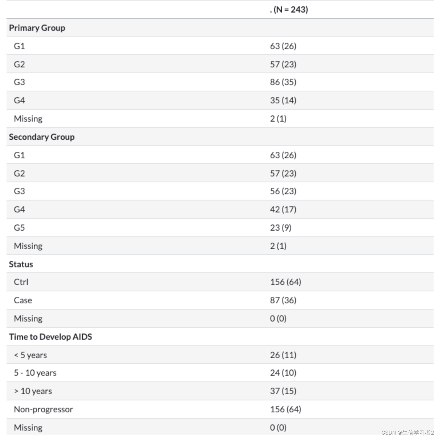
整理汇总表
# Tidy up the baseline data
df_v1 <- df_v1 %>%
  mutate(
    drink = case_when(
      drink %in% c("none", "low/moderate") ~ "low",
      drink %in% c("moderate/heavy", "binge") ~ "heavy",
      TRUE ~ "missing"
    )
  )

options(qwraps2_markup = "markdown")

summary_template <-
  list("Primary Group" =
         list("G1" = ~ n_perc0(group1 == "g1", na_rm = T),
              "G2" = ~ n_perc0(group1 == "g2", na_rm = T),
              "G3" = ~ n_perc0(group1 == "g3", na_rm = T),
              "G4" = ~ n_perc0(group1 == "g4", na_rm = T),
              "Missing" = ~ n_perc0(group1 == "missing", na_rm = T)),
       "Secondary Group" =
         list("G1" = ~ n_perc0(group2 == "g1", na_rm = T),
              "G2" = ~ n_perc0(group2 == "g2", na_rm = T),
              "G3" = ~ n_perc0(group2 == "g3", na_rm = T),
              "G4" = ~ n_perc0(group2 == "g4", na_rm = T),
              "G5" = ~ n_perc0(group2 == "g5", na_rm = T),
              "Missing" = ~ n_perc0(group2 == "missing", na_rm = T)),
       "Status" =
         list("Ctrl" = ~ n_perc0(status == "nc", na_rm = T),
              "Case" = ~ n_perc0(status == "sc", na_rm = T),
              "Missing" = ~ n_perc0(status == "missing", na_rm = T)),
       "Time to Develop AIDS" =
         list("< 5 years" = ~ n_perc0(time2aids == "< 5 yrs", na_rm = T),
              "5 - 10 years" = ~ n_perc0(time2aids == "5 - 10 yrs", na_rm = T),
              "> 10 years" = ~ n_perc0(time2aids == "> 10 yrs", na_rm = T),
              "Non-progressor" = ~ n_perc0(time2aids == "never", na_rm = T),
              "Missing" = ~ n_perc0(time2aids == "missing", na_rm = T)),
       "Age" =
         list("min" = ~ round(min(age, na.rm = T), 2),
              "max" = ~ round(max(age, na.rm = T), 2),
              "mean (sd)" = ~ qwraps2::mean_sd(age, na_rm = T, show_n = "never")),
       "Race" =
         list("White" = ~ n_perc0(race == "white", na_rm = T),
              "Black" = ~ n_perc0(race == "black", na_rm = T),
              "Others" = ~ n_perc0(race == "others", na_rm = T),
              "Missing" = ~ n_perc0(race == "missing", na_rm = T)),
       "Education" =
         list("Postgrad" = ~ n_perc0(educa == "postgrad", na_rm = T),
              "Undergrad" = ~ n_perc0(educa == "undergrad", na_rm = T),
              "No degree" = ~ n_perc0(educa == "no degree", na_rm = T),
              "Missing" = ~ n_perc0(educa == "missing", na_rm = T)),
       "Smoking status" =
         list("Never" = ~ n_perc0(smoke == "never", na_rm = T),
              "Former" = ~ n_perc0(smoke == "former", na_rm = T),
              "Current" = ~ n_perc0(smoke == "current", na_rm = T),
              "Missing" = ~ n_perc0(smoke == "missing", na_rm = T)),
       "Drinking status" =
         list("Low" = ~ n_perc0(drink == "low", na_rm = T),
              "Heavy" = ~ n_perc0(drink == "heavy", na_rm = T),
              "Missing" = ~ n_perc0(drink == "missing", na_rm = T)),
       "Antibiotics Usage" =
         list("No" = ~ n_perc0(abx_use == "no", na_rm = T),
              "Yes" = ~ n_perc0(abx_use == "yes", na_rm = T),
              "Missing" = ~ n_perc0(abx_use == "missing", na_rm = T)),
       "STD" =
         list("No" = ~ n_perc0(std == "no", na_rm = T),
              "Yes" = ~ n_perc0(std == "yes", na_rm = T),
              "Missing" = ~ n_perc0(std == "missing", na_rm = T)),
       "Substance use" =
         list("No" = ~ n_perc0(druguse == "no", na_rm = T),
              "Yes" = ~ n_perc0(druguse == "yes", na_rm = T),
              "Missing" = ~ n_perc0(druguse == "missing", na_rm = T)),
       "HBV" =
         list("Negative" = ~ n_perc0(hbv == "negative", na_rm = T),
              "Resolved" = ~ n_perc0(hbv == "resolved", na_rm = T),
              "Positive" = ~ n_perc0(hbv == "positive", na_rm = T),
              "Missing" = ~ n_perc0(hbv == "missing", na_rm = T)),
       "HCV" =
         list("Negative" = ~ n_perc0(hcv == "negative", na_rm = T),
              "Positive" = ~ n_perc0(hcv == "positive", na_rm = T),
              "Missing" = ~ n_perc0(hcv == "missing", na_rm = T))
  )

tab <- df_v1 %>%
  summary_table(summary_template)
# print(tab, rtitle = "Demographic information at the baseline visit")

knitr::kable(tab, caption = "Demographic information at the baseline visit")
Outcome vs. other variables
结局变量status(seroconverter (SC) rates 和 seronegative control (NC))与其他变量的相关关系,通过glm广义线性模型计算获得,并使用森林图展示结果。
df <- df_v1 %>%
  filter(!is.na(age), educa != "missing", abx_use != "missing",
         std != "missing", smoke != "missing", drink != "missing",
         druguse != "missing", hbv != "missing",
         status != "missing")
df$status <- factor(df$status, levels = c("nc", "sc"))
df$educa <- factor(df$educa, levels = c("no degree", "undergrad", "postgrad"))
df$abx_use <- factor(df$abx_use, levels = c("no", "yes"))
df$std <- factor(df$std, levels = c("no", "yes"))
df$smoke <- factor(df$smoke, levels = c("never", "former", "current"))
df$drink <- factor(df$drink, levels = c("low", "heavy"))
df$druguse <- factor(df$druguse, levels = c("no", "yes"))
df$hbv <- factor(df$hbv, levels = c("negative", "resolved", "positive"))

model <- glm(status ~ age + educa + abx_use + std + smoke + drink +
              druguse + hbv, data = df, family = binomial)

tidy_model <- broom::tidy(model) %>%
  filter(term != "(Intercept)") %>%
  mutate(index = seq_len(length(coef(model)) - 1),
         label = c("Age", "Educa (Undergrad)", "Educa (Postgrad)",
                   "Abx Use (Yes)", "STD (Yes)",
                   "Smoke (Former)", "Smoke (Current)",
                   "Drink (Heavy)", "Substance Use (Yes)",  "HBV (Resolved)", "HBV (Positive)"),
         label_factor = factor(label, levels = rev(sort(label))),
         p_value = round(p.value, 2),
         OR = exp(estimate),
         LL = exp(estimate - 1.96*std.error),
         UL = exp(estimate + 1.96*std.error)) %>%
  rowwise() %>%
  mutate(CI = paste(round(LL, 2), round(UL, 2), sep = ", ")) %>%
  ungroup()

p_forest <- tidy_model %>%
  ggplot(aes(y = label_factor, x = OR)) +
  geom_vline(xintercept = 1, color = "red", linetype = "dashed", linewidth = 1, alpha = 0.5) +
  geom_errorbarh(aes(xmin = LL, xmax = UL), height = 0.25) +
  geom_point(shape = 18, size = 5) +
  scale_x_log10(breaks = c(0.1, 0.2, 0.5, 1, 2, 5, 10),
                labels = c("0.1", "0.2", "0.5", "1", "2", "5", "10")) +
  scale_y_discrete(name = "") +
  labs(x = "Odds Ratio (95% CI)", y = "") +
  theme_bw() +
  theme(panel.border = element_blank(),
        panel.background = element_blank(),
        panel.grid.major = element_blank(),
        panel.grid.minor = element_blank(),
        axis.line = element_line(colour = "black"),
        axis.text.y = element_text(size = 12, colour = "black"),
        axis.text.x.bottom = element_text(size = 12, colour = "black"),
        axis.title.x = element_text(size = 12, colour = "black")) +
  ggtitle("")

table_base <- tidy_model %>%
  ggplot(aes(y = label_factor)) +
  labs(x = "", y = "") +
  theme(plot.title = element_text(hjust = 0.5, size = 12),
        axis.text.x = element_text(color = "white", hjust = -3, size = 25),
        axis.line = element_blank(),
        axis.text.y = element_blank(),
        axis.ticks = element_blank(),
        axis.title.y = element_blank(),
        legend.position = "none",
        panel.background = element_blank(),
        panel.border = element_blank(),
        panel.grid.major = element_blank(),
        panel.grid.minor = element_blank(),
        plot.background = element_blank())

tab_or <- table_base +
  geom_text(aes(y = label_factor, x = 1,
                label = sprintf("%0.1f", round(OR, digits = 1))), size = 4) +
  ggtitle("OR")

tab_ci <- table_base +
  geom_text(aes(y = label_factor, x = 1, label = CI), size = 4) +
  ggtitle("95% CI")

tab_p <- table_base +
  geom_text(aes(y = label_factor, x = 1, label = p_value), size = 4) +
  ggtitle("P")

p_out_var_prim <- ggarrange(
  p_forest, tab_or, tab_ci, tab_p,
  ncol = 4, nrow = 1,
  widths = c(10, 1, 2, 1), align = "h")

p_out_var_prim
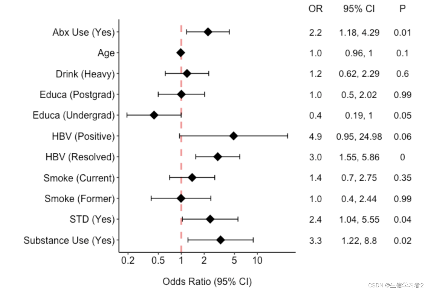
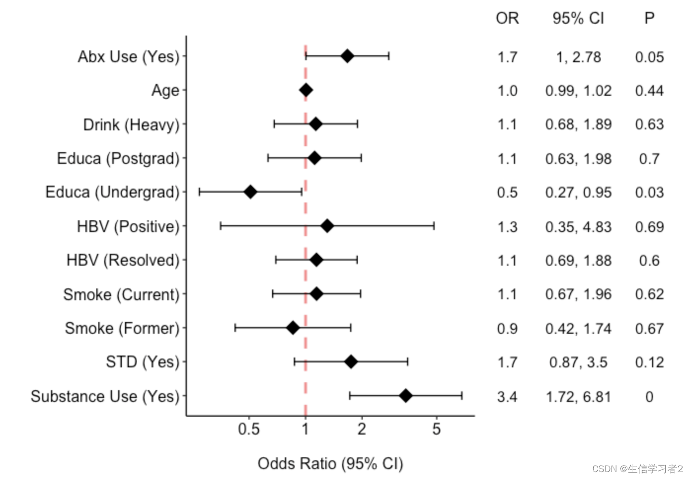
结果:森林图展示其他变量与结局变量status的相关关系
-
“Abx Use (Yes)” 的OR为2.2,95% CI为1.18到4.29,P值为0.01,表示使用抗生素与结果的关联是显著的,使用抗生素的人发生结果的可能性大约是不使用的人的2.2倍。
-
“Educa (Undergrad)” 的OR为0.4,95% CI为0.19到1,P值为0.05,表示拥有本科教育的人发生结果的可能性大约是未受本科教育的人的0.4倍,这个关联在统计学上也是显著的。
-
“HBV (Resolved)” 的OR为3.0,95% CI为1.55到5.86,P < 0.05,表示HBV(乙型肝炎病毒)已解决的个体发生结果的可能性是未解决的个体的3倍,这个关联非常显著。
-
“Substance Use (Yes)” 的OR为3.3,95% CI为1.22到8.8,P值为0.02,表示有物质使用的人发生结果的可能性大约是不使用物质的人的3.3倍,这个关联也是显著的。
Exposure (primary group) vs. outcome
使用Constrained Inference for Linear Mixed Effects Models(线性混合效应模型的约束推理)方法解析primary group变量和status结局变量的关系。
线性混合效应模型(Linear Mixed-Effects Models,简称LMMs)是一种用于分析具有多层次或嵌套结构数据的统计模型。这种模型可以处理数据中的固定效应(fixed effects)和随机效应(random effects),使得研究者能够考虑和控制数据中的非独立性(non-independence)。在传统的线性模型中,参数估计通常是通过最小化残差平方和来完成的,这被称为无约束估计(unconstrained estimation)。然而,在某些情况下,我们可能希望对模型参数施加一些约束条件,比如参数的正性、非负性或其他类型的线性约束。这就是所谓的约束推理。
与传统线性模型的不同。
-
处理复杂数据结构:LMMs可以处理具有多层次或嵌套结构的数据,而传统线性模型通常假设数据是独立的。
-
灵活性:LMMs通过固定效应和随机效应的结合,提供了更大的灵活性来捕捉数据中的复杂关系。
-
参数约束:在约束推理中,LMMs可以对参数施加特定的约束,这在传统线性模型中不常见。
-
估计方法:LMMs可能需要更复杂的估计方法,如最大似然估计、贝叶斯方法或限制性最大似然估计,以处理随机效应。
-
计算复杂性:由于需要估计额外的随机效应参数,LMMs的计算通常比传统线性模型更为复杂。
df_fig <- df_v1 %>%
  filter(group1 != "missing",
         status != "missing") %>%
  group_by(group1) %>%
  summarise(total = n(),
            nc_num = sum(status == "nc"),
            sc_num = sum(status == "sc")) %>%
  dplyr::mutate(perc_nc = round(nc_num/total * 100, 2),
                perc_sc = round(sc_num/total * 100, 2)) %>%
  dplyr::select(group1, perc_nc, perc_sc) %>%
  pivot_longer(cols = perc_nc:perc_sc, names_to = "perc", values_to = "value")

cons <- list(order = "simple", decreasing = FALSE, node = 1)
df_test <- df_v1 %>%
  filter(group1 != "missing",
         status != "missing") %>%
  transmute(group1 = group1,
            status = ifelse(status == "nc", 0, 1))
df_test$group1 <- factor(df_test$group1, ordered = TRUE)
fit_clme <- clme(status ~ group1, data = df_test, constraints = cons, seed = 123)
fit_summ <- summary(fit_clme)

fit_summ

p_val <- fit_summ$p.value
p_lab <- ifelse(p_val == 0, "p < 0.001", paste0("p = ", p_val))
test_lab <- paste0("LRT = ", signif(fit_summ$ts.glb, 2))
lab <- paste0(test_lab, ", ", p_lab)

df_fig$group1 <- recode(df_fig$group1,
                       `g1` = "G1", `g2` = "G2",
                       `g3` = "G3", `g4` = "G4")

p_summ_prim <- df_fig %>%
  ggbarplot(x = "group1", y = "value",
            fill = "perc", color = "black", palette = "Paired",
            xlab = "", ylab = "Percentage (%)",
            label = TRUE, lab.col = "white", lab.pos = "in") +
  scale_y_continuous(breaks = c(0, 20, 40, 60, 80, 100), limits = c(0, 110)) +
  geom_text(aes(x = 3.5, y = 110, label = lab)) +
  scale_fill_aaas(name = NULL, labels = c("Ctrl", "Case"))

p_summ_prim
Linear mixed model subject to order restrictions
Formula: status ~ group1 - 1

Order specified: increasing simple order

log-likelihood: -134.1
AIC:             278.1
BIC:             286.4
(log-likelihood, AIC, BIC computed under normality)

Global test:
 Contrast       Statistic  p-value
 Bootstrap LRT      0.002   0.0000

Individual Tests (Williams' type tests):
 Contrast  Estimate  Statistic  p-value
 g2 - g1      0.251      3.249   0.0000
 g3 - g2      0.178      2.476   0.0000
 g4 - g3      0.266      3.145   0.0000

Variance components:
         Std. Error
Residual   0.422039

Fixed effect coefficients (theta):
     Estimate  Std. Err  95% lower  95% upper
 g1   0.04762   0.05317     -0.057      0.152
 g2   0.29825   0.05590      0.189      0.408
 g3   0.47674   0.04551      0.388      0.566
 g4   0.74286   0.07134      0.603      0.883
Std. Errors and confidence limits based on unconstrained covariance matrix

Parameters are ordered according to the following factor levels:
g1, g2, g3, g4
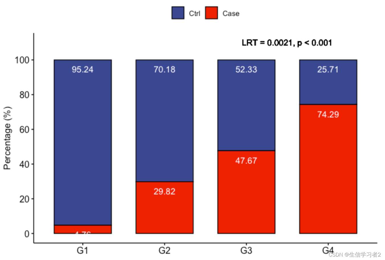
结果:Constrained Inference for Linear Mixed Effects Models的结果(排序)
-
LRT(Likelihood Ratio Test):似然比检验是一种统计假设检验方法,用于比较两个嵌套模型的拟合优度。
-
由于LRT的P值非常小,这表明在模型中考虑排序约束是合理的,即模型的复杂版本(包含排序约束)比简单版本提供了显著更好的拟合。
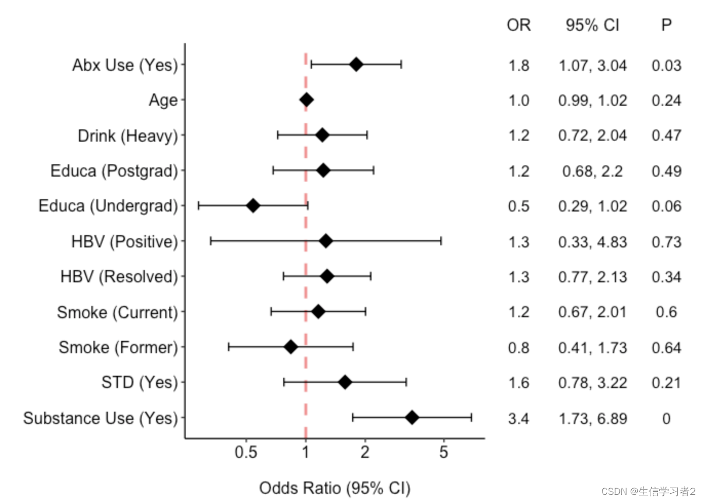
Exposure (primary group) vs. other variables
暴露变量Exposure (primary group)与其他变量的相关关系,通过Ordered Logistic or Probit Regression线性模型计算获得,并使用森林图展示结果。
Ordered Logistic Regression(有序逻辑回归)和Ordered Probit Regression(有序Probit回归)是两种用于分析有序分类数据的统计方法。有序分类数据是指数据的类别具有自然的顺序或等级,例如,调查问卷中的满意度评级(非常不满意、不满意、一般、满意、非常满意)。
-
有序逻辑回归是一种广义线性模型(Generalized Linear Model, GLM),它使用逻辑函数(通常是Logit函数)来连接预测变量和有序类别的累积概率。
-
有序Probit回归与有序逻辑回归类似,但它使用正态分布的累积分布函数(CDF)作为连接函数,而不是逻辑函数。
df <- df_v1 %>%
  filter(!is.na(age), educa != "missing", abx_use != "missing",
         std != "missing", smoke != "missing", drink != "missing",
         druguse != "missing", hbv != "missing",
         group1 != "missing")
df$group1 <- factor(df$group1, levels = c("g1", "g2", "g3", "g4"))
df$educa <- factor(df$educa, levels = c("no degree", "undergrad", "postgrad"))
df$abx_use <- factor(df$abx_use, levels = c("no", "yes"))
df$std <- factor(df$std, levels = c("no", "yes"))
df$smoke <- factor(df$smoke, levels = c("never", "former", "current"))
df$drink <- factor(df$drink, levels = c("low", "heavy"))
df$druguse <- factor(df$druguse, levels = c("no", "yes"))
df$hbv <- factor(df$hbv, levels = c("negative", "resolved", "positive"))

model <- polr(group1 ~ age + educa + abx_use + std + smoke + drink +
              druguse + hbv, data = df, Hess = TRUE, method = "logistic")

coefs <- summary(model)$coefficients
wald_stat <- coefs[, "Value"] / coefs[, "Std. Error"]
wald_pvalue <- 2 * pnorm(abs(wald_stat), lower.tail = FALSE)
wald_pvalue <- wald_pvalue[!names(wald_pvalue) %in% c("g1|g2", "g2|g3", "g3|g4")]

tidy_model <- broom::tidy(model) %>%
  filter(!term %in% c("g1|g2", "g2|g3", "g3|g4")) %>%
  mutate(label = c("Age", "Educa (Undergrad)", "Educa (Postgrad)",
                   "Abx Use (Yes)", "STD (Yes)",
                   "Smoke (Former)", "Smoke (Current)",
                   "Drink (Heavy)", "Substance Use (Yes)", "HBV (Resolved)", "HBV (Positive)"),
         label_factor = factor(label, levels = rev(sort(label))),
         p_value = round(wald_pvalue, 2),
         OR = exp(estimate),
         LL = exp(estimate - 1.96*std.error),
         UL = exp(estimate + 1.96*std.error)) %>%
  rowwise() %>%
  mutate(CI = paste(round(LL, 2), round(UL, 2), sep = ", ")) %>%
  ungroup()

p_forest <- tidy_model %>%
  ggplot(aes(y = label_factor, x = OR)) +
  geom_vline(xintercept = 1, color = "red", linetype = "dashed", cex = 1, alpha = 0.5) +
  geom_errorbarh(aes(xmin = LL, xmax = UL), height = 0.25) +
  geom_point(shape = 18, size = 5) +
  scale_x_log10(breaks = c(0.1, 0.2, 0.5, 1, 2, 5, 10),
                labels = c("0.1", "0.2", "0.5", "1", "2", "5", "10")) +
  scale_y_discrete(name = "") +
  labs(x = "Odds Ratio (95% CI)", y = "") +
  theme_bw() +
  theme(panel.border = element_blank(),
        panel.background = element_blank(),
        panel.grid.major = element_blank(),
        panel.grid.minor = element_blank(),
        axis.line = element_line(colour = "black"),
        axis.text.y = element_text(size = 12, colour = "black"),
        axis.text.x.bottom = element_text(size = 12, colour = "black"),
        axis.title.x = element_text(size = 12, colour = "black")) +
  ggtitle("")

table_base <- tidy_model %>%
  ggplot(aes(y = label_factor)) +
  labs(x = "", y = "") +
  theme(plot.title = element_text(hjust = 0.5, size = 12),
        axis.text.x = element_text(color = "white", hjust = -3, size = 25),
        axis.line = element_blank(),
        axis.text.y = element_blank(),
        axis.ticks = element_blank(),
        axis.title.y = element_blank(),
        legend.position = "none",
        panel.background = element_blank(),
        panel.border = element_blank(),
        panel.grid.major = element_blank(),
        panel.grid.minor = element_blank(),
        plot.background = element_blank())

tab_or <- table_base +
  geom_text(aes(y = label_factor, x = 1,
                label = sprintf("%0.1f", round(OR, digits = 1))), size = 4) +
  ggtitle("OR")

tab_ci <- table_base +
  geom_text(aes(y = label_factor, x = 1, label = CI), size = 4) +
  ggtitle("95% CI")

tab_p <- table_base +
  geom_text(aes(y = label_factor, x = 1, label = p_value), size = 4) +
  ggtitle("P")

p_exp_var_prim <- ggarrange(
  p_forest, tab_or, tab_ci, tab_p,
  ncol = 4, nrow = 1,
  widths = c(10, 1, 2, 1), align = "h")

p_exp_var_prim
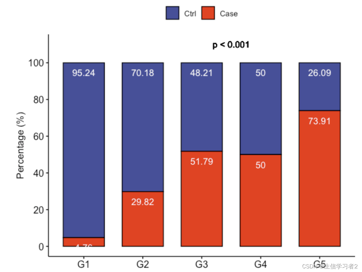
Exposure (secondary group) vs. outcome
使用Constrained Inference for Linear Mixed Effects Models(线性混合效应模型的约束推理)方法解析secondary group变量和status结局变量的关系。
df_fig <- df_v1 %>%
  filter(group2 != "missing",
         status != "missing") %>%
  group_by(group2) %>%
  summarise(total = n(),
            nc_num = sum(status == "nc"),
            sc_num = sum(status == "sc")) %>%
  dplyr::mutate(perc_nc = round(nc_num/total * 100, 2),
                perc_sc = round(sc_num/total * 100, 2)) %>%
  dplyr::select(group2, perc_nc, perc_sc) %>%
  pivot_longer(cols = perc_nc:perc_sc, names_to = "perc", values_to = "value")

cons <- list(order = "simple", decreasing = FALSE, node = 1)
df_test <- df_v1 %>%
  filter(group2 != "missing",
         status != "missing") %>%
  transmute(group2 = group2,
            status = ifelse(status == "nc", 0, 1))
df_test$group2 <- factor(df_test$group2, ordered = TRUE)
fit_clme <- clme(status ~ group2, data = df_test, constraints = cons, seed = 123)
fit_summ <- summary(fit_clme)

fit_summ

p_val <- fit_summ$p.value
p_lab <- ifelse(p_val == 0, "p < 0.001", paste0("p = ", p_val))

df_fig$group2 <- recode(df_fig$group2,
                       `g1` = "G1", `g2` = "G2",
                       `g3` = "G3", `g4` = "G4", `g5` = "G5")

p_summ_second <- df_fig %>%
  ggbarplot(x = "group2", y = "value",
            fill = "perc", color = "black", palette = "Paired",
            xlab = "", ylab = "Percentage (%)",
            label = TRUE, lab.col = "white", lab.pos = "in") +
  scale_y_continuous(breaks = c(0, 20, 40, 60, 80, 100), limits = c(0, 110)) +
  geom_text(aes(x = 3.5, y = 110, label = p_lab)) +
  scale_fill_aaas(name = NULL, labels = c("Ctrl", "Case"))

p_summ_second
Linear mixed model subject to order restrictions
Formula: status ~ group2 - 1

Order specified: increasing simple order

log-likelihood: -136.2
AIC:             284.5
BIC:             294.4
(log-likelihood, AIC, BIC computed under normality)

Global test:
 Contrast       Statistic  p-value
 Bootstrap LRT      0.003   0.0000

Individual Tests (Williams' type tests):
 Contrast  Estimate  Statistic  p-value
 g2 - g1      0.251      3.219   0.0000
 g3 - g2      0.212      2.645   0.0000
 g4 - g3      0.000      0.000   1.0000
 g5 - g4      0.229      2.072   0.0050

Variance components:
         Std. Error
Residual  0.4258823

Fixed effect coefficients (theta):
     Estimate  Std. Err  95% lower  95% upper
 g1   0.04762   0.05366     -0.058      0.153
 g2   0.29825   0.05641      0.188      0.409
 g3   0.51020   0.05691      0.399      0.622
 g4   0.51020   0.06572      0.381      0.639
 g5   0.73913   0.08880      0.565      0.913
Std. Errors and confidence limits based on unconstrained covariance matrix

Parameters are ordered according to the following factor levels:
g1, g2, g3, g4, g5
Exposure (secondary group) vs. other variables
df <- df_v1 %>%
  filter(!is.na(age), educa != "missing", abx_use != "missing",
         std != "missing", smoke != "missing", drink != "missing",
         druguse != "missing", hbv != "missing",
         group2 != "missing")
df$group2 <- factor(df$group2, levels = c("g1", "g2", "g3", "g4", "g5"))
df$educa <- factor(df$educa, levels = c("no degree", "undergrad", "postgrad"))
df$abx_use <- factor(df$abx_use, levels = c("no", "yes"))
df$std <- factor(df$std, levels = c("no", "yes"))
df$smoke <- factor(df$smoke, levels = c("never", "former", "current"))
df$drink <- factor(df$drink, levels = c("low", "heavy"))
df$druguse <- factor(df$druguse, levels = c("no", "yes"))
df$hbv <- factor(df$hbv, levels = c("negative", "resolved", "positive"))

model <- polr(group2 ~ age + educa + abx_use + std + smoke + drink +
              druguse + hbv, data = df, Hess = TRUE, method = "logistic")

coefs <- summary(model)$coefficients
wald_stat <- coefs[, "Value"] / coefs[, "Std. Error"]
wald_pvalue <- 2 * pnorm(abs(wald_stat), lower.tail = FALSE)
wald_pvalue <- wald_pvalue[!names(wald_pvalue) %in% c("g1|g2", "g2|g3", "g3|g4", "g4|g5")]

tidy_model <- broom::tidy(model) %>%
  filter(!term %in% c("g1|g2", "g2|g3", "g3|g4", "g4|g5")) %>%
  mutate(label = c("Age", "Educa (Undergrad)", "Educa (Postgrad)",
                   "Abx Use (Yes)", "STD (Yes)",
                   "Smoke (Former)", "Smoke (Current)",
                   "Drink (Heavy)", "Substance Use (Yes)", "HBV (Resolved)", "HBV (Positive)"),
         label_factor = factor(label, levels = rev(sort(label))),
         p_value = round(wald_pvalue, 2),
         OR = exp(estimate),
         LL = exp(estimate - 1.96*std.error),
         UL = exp(estimate + 1.96*std.error)) %>%
  rowwise() %>%
  mutate(CI = paste(round(LL, 2), round(UL, 2), sep = ", ")) %>%
  ungroup()

p_forest <- tidy_model %>%
  ggplot(aes(y = label_factor, x = OR)) +
  geom_vline(xintercept = 1, color = "red", linetype = "dashed", cex = 1, alpha = 0.5) +
  geom_errorbarh(aes(xmin = LL, xmax = UL), height = 0.25) +
  geom_point(shape = 18, size = 5) +
  scale_x_log10(breaks = c(0.1, 0.2, 0.5, 1, 2, 5, 10),
                labels = c("0.1", "0.2", "0.5", "1", "2", "5", "10")) +
  scale_y_discrete(name = "") +
  labs(x = "Odds Ratio (95% CI)", y = "") +
  theme_bw() +
  theme(panel.border = element_blank(),
        panel.background = element_blank(),
        panel.grid.major = element_blank(),
        panel.grid.minor = element_blank(),
        axis.line = element_line(colour = "black"),
        axis.text.y = element_text(size = 12, colour = "black"),
        axis.text.x.bottom = element_text(size = 12, colour = "black"),
        axis.title.x = element_text(size = 12, colour = "black")) +
  ggtitle("")

table_base <- tidy_model %>%
  ggplot(aes(y = label_factor)) +
  labs(x = "", y = "") +
  theme(plot.title = element_text(hjust = 0.5, size = 12),
        axis.text.x = element_text(color = "white", hjust = -3, size = 25),
        axis.line = element_blank(),
        axis.text.y = element_blank(),
        axis.ticks = element_blank(),
        axis.title.y = element_blank(),
        legend.position = "none",
        panel.background = element_blank(),
        panel.border = element_blank(),
        panel.grid.major = element_blank(),
        panel.grid.minor = element_blank(),
        plot.background = element_blank())

tab_or <- table_base +
  geom_text(aes(y = label_factor, x = 1,
                label = sprintf("%0.1f", round(OR, digits = 1))), size = 4) +
  ggtitle("OR")

tab_ci <- table_base +
  geom_text(aes(y = label_factor, x = 1, label = CI), size = 4) +
  ggtitle("95% CI")

tab_p <- table_base +
  geom_text(aes(y = label_factor, x = 1, label = p_value), size = 4) +
  ggtitle("P")

p_exp_var_second <- ggarrange(
  p_forest, tab_or, tab_ci, tab_p,
  ncol = 4, nrow = 1,
  widths = c(10, 1, 2, 1), align = "h")

p_exp_var_second


 791
791


 被折叠的 条评论
为什么被折叠?
被折叠的 条评论
为什么被折叠?
 到【灌水乐园】发言


