


介绍
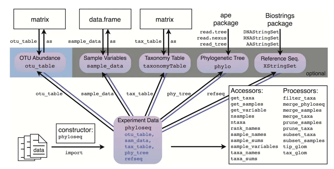
phyloseq包对多类型数据的综合软件,并其对这些数据提供统计分析和可视化方法。
微生物数据分析的主要挑战之一是如何整合不同类型的数据,从而对其进行生态学、遗传学、系统发育学、多元统计、可视化和检验等分析。同时,由于同行之间需要分享彼此的分析结果,如何去重复各自的结果呢?这需要一款统一数据输入接口且包含多种分析方法的软件,而phyloseq就是为处理这样的问题诞生的R包。
phyloseq数据结构
phyloseq对象的输入数据:
- **otu_table:**也即是物种丰度表,以matrix方式输入,行名是物种名字;
- **sample_data:**表型数据,包含样本的分组信息和环境因素等,以data.frame方式输入,行名是样本名字;
- tax_table:物种分类学水平的信息,以matrix方式输入,行名或者第一列是otu_table的行名;
- **phy_tree:**OTU的进化树关系表,计算uniFrac距离;
- refseq: DNA,RNA和AA氨基酸的序列信息。
使用
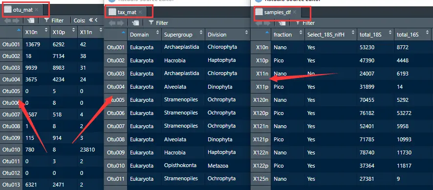
输入数据
- 物种丰度表: otu_mat
- 物种分类水平表:tax_mat
- 样本表型:samples_df
library(dplyr)
library(ggplot2)
library(phyloseq)
library(readxl)
library(tibble)

otu_mat<- read_excel("../datset/CARBOM data.xlsx", sheet = "OTU matrix") %>% column_to_rownames("otu")
tax_mat<- read_excel("../datset/CARBOM data.xlsx", sheet = "Taxonomy table") %>% column_to_rownames("otu")
samples_df <- read_excel("../datset/CARBOM data.xlsx", sheet = "Samples") %>% column_to_rownames("sample")
OTU <- otu_table(otu_mat %>% as.matrix(), taxa_are_rows = TRUE)
TAX <- tax_table(tax_mat %>% as.matrix())
samples <- sample_data(samples_df)

carbom <- phyloseq(OTU, TAX, samples)
对phylose对象的处理
# 数据名字
sample_names(carbom)
rank_names(carbom)
sample_variables(carbom)

# 数据子集
subset_samples(carbom, Select_18S_nifH =="Yes")
subset_taxa(carbom, Division %in% c("Chlorophyta", "Dinophyta", "Cryptophyta",
                                                "Haptophyta", "Ochrophyta", "Cercozoa"))
subset_taxa(carbom, !(Class %in% c("Syndiniales", "Sarcomonadea")))

# 中位数测序深度归一化reads数目
total <- median(sample_sums(carbom))
standf <- function(x, t=total){round(t * (x / sum(x)))}
carbom <- transform_sample_counts(carbom, standf)
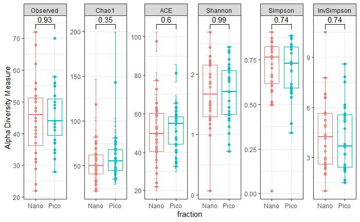
alpha diversity
plot_richness(carbom, x="fraction", color = "fraction",
                    measures=c("Observed", "Chao1", "ACE", "Shannon", "Simpson", "InvSimpson"))+
  stat_boxplot(geom='errorbar', linetype=1, width=0.3)+
  geom_boxplot(aes(color=fraction), alpha=0.1)+
  ggpubr::stat_compare_means(comparisons = list(c("Nano", "Pico")),
                             method = "wilcox.test")+
  guides(color=F)+
  theme_bw()
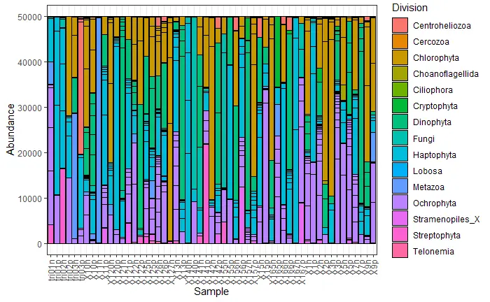
barplot
plot_bar(carbom, fill = "Division")+
  theme_bw()+
  # 0->left; .5->center; 1->right
  theme(axis.text.x = element_text(angle = 90, vjust = .5, hjust = 1))
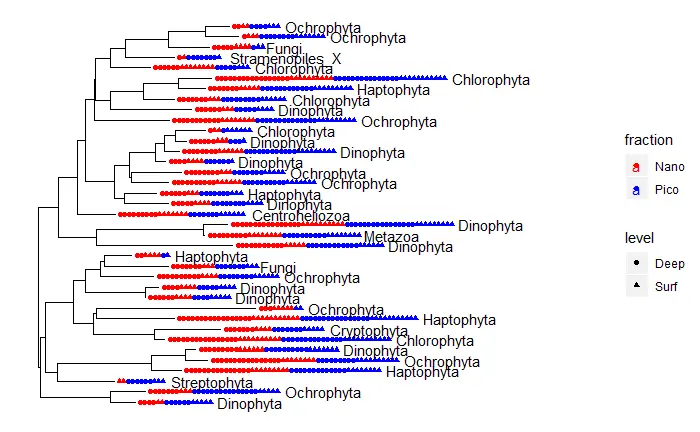
tree
library(ape)
random_tree <- rtree(ntaxa(carbom), rooted=TRUE, tip.label=taxa_names(carbom))
carbom_tree <- phyloseq(OTU, TAX, samples, random_tree)

#  at least 20% of reads in at least one sample
carbom_abund <- filter_taxa(carbom_tree, function(x) {sum(x > total*0.20) > 0}, TRUE)

plot_tree(carbom_abund, color="fraction", shape="level", label.tips="Division", ladderize="left", plot.margin=0.3)+
  labs(x="",y="")+
  scale_color_manual(values = c("red", "blue"))+
  theme_bw()
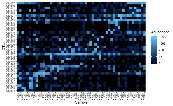
heatmap
#  at least 20% of reads in at least one sample
carbom_abund <- filter_taxa(carbom_tree, function(x) {sum(x > total*0.20) > 0}, TRUE)
plot_heatmap(carbom_abund, method = "NMDS", distance = "bray")

# 自己设定距离
# plot_heatmap(carbom_abund, method = "MDS", distance = "(A+B-2*J)/(A+B-J)",
#                taxa.label = "Class", taxa.order = "Class",
#                trans=NULL, low="beige", high="red", na.value="beige")
For vectors x and y the “quadratic” terms are J = sum(x*y), A = sum(x^2), B = sum(y^2) and “minimum” terms are J = sum(pmin(x,y)), A = sum(x) and B = sum(y), and “binary” terms are either of these after transforming data into binary form (shared number of species, and number of species for each row). Somes examples :
- A+B-2*J “quadratic” squared Euclidean
- A+B-2*J “minimum” Manhattan
- (A+B-2*J)/(A+B) “minimum” Bray-Curtis
- (A+B-2*J)/(A+B) “binary” Sørensen
- (A+B-2*J)/(A+B-J) “binary” Jaccard
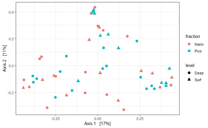
ordination
# method : c("DCA", "CCA", "RDA", "CAP", "DPCoA", "NMDS", "MDS", "PCoA")
# disrance: unlist(distanceMethodList)
carbom.ord <- ordinate(carbom, method = "PCoA", distance = "bray")

# plot_ordination(carbom, carbom.ord, type="taxa", color="Class", shape= "Class",
#                   title="OTUs")

plot_ordination(carbom, carbom.ord, type="samples", color="fraction",
                  shape="level")+
  geom_point(size=3)+
  theme_bw()
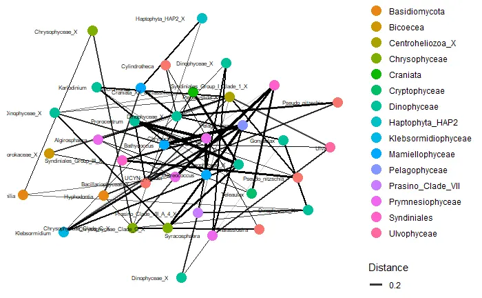
network analysis
# plot_net(carbom, distance = "(A+B-2*J)/(A+B)", type = "taxa",
#           maxdist = 0.7, color="Class", point_label="Genus")

# plot_net(carbom, distance = "(A+B-2*J)/(A+B)", type = "samples",
#            maxdist = 0.7, color="fraction", point_label="fraction")

plot_net(carbom_abund, distance = "(A+B-2*J)/(A+B)", type = "taxa",
           maxdist = 0.8, color="Class", point_label="Genus")
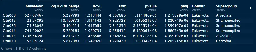
Deseq2 with phyloseq
library(DESeq2)
library(ggplot2)

diagdds <- phyloseq_to_deseq2(carbom_abund, ~ fraction)
diagdds <- DESeq(diagdds, test="Wald", fitType="parametric")

res <- results(diagdds, cooksCutoff = FALSE)
sigtab <- res[which(res$padj < 0.01), ]
sigtab <- cbind(as(sigtab, "data.frame"), as(tax_table(carbom_abund)[rownames(sigtab), ], "matrix"))
head(sigtab)
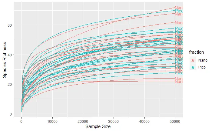
rarefaction curves
rarecurve2 <- function (x, step = 1, sample, xlab = "Sample Size", ylab = "Species", label = TRUE, col = "black", ...)
  ## See documentation for vegan rarecurve, col is now used to define
  ## custom colors for lines and panels
{
  tot <- rowSums(x)
  S <- vegan::specnumber(x)
  nr <- nrow(x)
  out <- lapply(seq_len(nr), function(i) {
    n <- seq(1, tot[i], by = step)
    if (n[length(n)] != tot[i])
      n <- c(n, tot[i])
    drop(vegan::rarefy(x[i, ], n))
  })
  Nmax <- sapply(out, function(x) max(attr(x, "Subsample")))
  Smax <- sapply(out, max)
  plot(c(1, max(Nmax)), c(1, max(Smax)), xlab = xlab, ylab = ylab,
       type = "n", ...)
  if (!missing(sample)) {
    abline(v = sample)
    rare <- sapply(out, function(z) approx(x = attr(z, "Subsample"),
                                           y = z, xout = sample, rule = 1)$y)
    abline(h = rare, lwd = 0.5)
  }
  for (ln in seq_len(length(out))) {
    color <- col[((ln-1) %% length(col)) + 1]
    N <- attr(out[[ln]], "Subsample")
    lines(N, out[[ln]], col = color, ...)
  }
  if (label) {
    ordilabel(cbind(tot, S), labels = rownames(x), col = col, ...)
  }
  invisible(out)
}

## Rarefaction curve, ggplot style
ggrare <- function(physeq, step = 10, label = NULL, color = NULL, plot = TRUE, parallel = FALSE, se = TRUE) {
  ## Args:
  ## - physeq: phyloseq class object, from which abundance data are extracted
  ## - step: Step size for sample size in rarefaction curves
  ## - label: Default `NULL`. Character string. The name of the variable
  ##          to map to text labels on the plot. Similar to color option
  ##          but for plotting text.
  ## - color: (Optional). Default ‘NULL’. Character string. The name of the
  ##          variable to map to colors in the plot. This can be a sample
  ##          variable (among the set returned by
  ##          ‘sample_variables(physeq)’ ) or taxonomic rank (among the set
  ##          returned by ‘rank_names(physeq)’).
  ##
  ##          Finally, The color scheme is chosen automatically by
  ##          ‘link{ggplot}’, but it can be modified afterward with an
  ##          additional layer using ‘scale_color_manual’.
  ## - color: Default `NULL`. Character string. The name of the variable
  ##          to map to text labels on the plot. Similar to color option
  ##          but for plotting text.
  ## - plot:  Logical, should the graphic be plotted.
  ## - parallel: should rarefaction be parallelized (using parallel framework)
  ## - se:    Default TRUE. Logical. Should standard errors be computed.
  ## require vegan
  x <- as(otu_table(physeq), "matrix")
  if (taxa_are_rows(physeq)) { x <- t(x) }

  ## This script is adapted from vegan `rarecurve` function
  tot <- rowSums(x)
  S <- rowSums(x > 0)
  nr <- nrow(x)

  rarefun <- function(i) {
    cat(paste("rarefying sample", rownames(x)[i]), sep = "\n")
    n <- seq(1, tot[i], by = step)
    if (n[length(n)] != tot[i]) {
      n <- c(n, tot[i])
    }
    y <- vegan::rarefy(x[i, ,drop = FALSE], n, se = se)
    if (nrow(y) != 1) {
      rownames(y) <- c(".S", ".se")
      return(data.frame(t(y), Size = n, Sample = rownames(x)[i]))
    } else {
      return(data.frame(.S = y[1, ], Size = n, Sample = rownames(x)[i]))
    }
  }
  if (parallel) {
    out <- mclapply(seq_len(nr), rarefun, mc.preschedule = FALSE)
  } else {
    out <- lapply(seq_len(nr), rarefun)
  }
  df <- do.call(rbind, out)

  ## Get sample data
  if (!is.null(sample_data(physeq, FALSE))) {
    sdf <- as(sample_data(physeq), "data.frame")
    sdf$Sample <- rownames(sdf)
    data <- merge(df, sdf, by = "Sample")
    labels <- data.frame(x = tot, y = S, Sample = rownames(x))
    labels <- merge(labels, sdf, by = "Sample")
  }

  ## Add, any custom-supplied plot-mapped variables
  if( length(color) > 1 ){
    data$color <- color
    names(data)[names(data)=="color"] <- deparse(substitute(color))
    color <- deparse(substitute(color))
  }
  if( length(label) > 1 ){
    labels$label <- label
    names(labels)[names(labels)=="label"] <- deparse(substitute(label))
    label <- deparse(substitute(label))
  }

  p <- ggplot(data = data, aes_string(x = "Size", y = ".S", group = "Sample", color = color))
  p <- p + labs(x = "Sample Size", y = "Species Richness")
  if (!is.null(label)) {
    p <- p + geom_text(data = labels, aes_string(x = "x", y = "y", label = label, color = color),
                       size = 4, hjust = 0)
  }
  p <- p + geom_line()
  if (se) { ## add standard error if available
    p <- p + geom_ribbon(aes_string(ymin = ".S - .se", ymax = ".S + .se", color = NULL, fill = color), alpha = 0.2)
  }
  if (plot) {
    plot(p)
  }
  invisible(p)
}

ggrare(carbom, step = 100, color = "fraction", label = "fraction", se = FALSE)
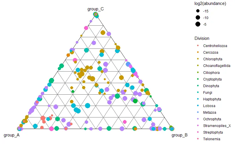
ternary
ternary_norm <- function(physeq, group, levelOrder = NULL, raw = FALSE, normalizeGroups = TRUE) {
    ## Args:
    ## - phyloseq class object, otus abundances are extracted from this object
    ## - group: Either the a single character string matching a
    ##          variable name in the corresponding sample_data of ‘physeq’, or a
    ##          factor with the same length as the number of samples in ‘physeq’.
    ## - raw: logical, should raw read counts be used to compute relative abudances of an
    ##        OTU among different conditions (defaults to FALSE)
    ## - levelOrder: Order along which to rearrange levels of `group`. Goes like (left, top, right) for
    ##               ternary plots and (left, top, right, bottom) for diamond plots.
    ## - normalizeGroups: logical, only used if raw = FALSE, should all levels be given
    ##                    equal weights (TRUE, default) or weights equal to their sizes (FALSE)

    ## Get grouping factor
    if (!is.null(sam_data(physeq, FALSE))) {
        if (class(group) == "character" & length(group) == 1) {
            x1 <- data.frame(sam_data(physeq))
            if (!group %in% colnames(x1)) {
                stop("group not found among sample variable names.")
            }
            group <- x1[, group]
        }
    }
    if (class(group) != "factor") {
        group <- factor(group)
    }

    ## Reorder levels of factor
    if (length(levels(group)) > 4) {
        warnings("There are 5 groups or more, the data frame will not be suitable for ternary plots.")
    }
    if (!is.null(levelOrder)) {
        if (any(! group %in% levelOrder)) {
            stop("Some levels of the factor are not included in `levelOrder`")
        } else {
            group <- factor(group, levels = levelOrder)
        }
    }

    ## construct relative abundances matrix
    tdf <- as(otu_table(physeq), "matrix")
    if (!taxa_are_rows(physeq)) { tdf <- t(tdf) }

    ## If raw, no normalisation should be done
    if (raw) {
        tdf <- t(tdf)
        abundance <- rowSums(t(tdf))/sum(tdf)
        meandf <- t(rowsum(tdf, group, reorder = TRUE))/rowSums(t(tdf))
    } else {
        ## Construct relative abundances by sample
        tdf <- apply(tdf, 2, function(x) x/sum(x))
        if (normalizeGroups) {
            meandf <- t(rowsum(t(tdf), group, reorder = TRUE)) / matrix(rep(table(group), each = nrow(tdf)),
                                                  nrow = nrow(tdf))
            abundance <- rowSums(meandf)/sum(meandf)
            meandf <- meandf / rowSums(meandf)
        } else {
            abundance <- rowSums(tdf)/sum(tdf)
            meandf <- t(rowsum(t(tdf), group, reorder = TRUE))/rowSums(tdf)
        }
    }

    ## Construct cartesian coordinates for de Finetti's diagram
    ## (taken from wikipedia, http://en.wikipedia.org/wiki/Ternary_plot)
    if (ncol(meandf) == 3) {
        ternary.coord <- function(a,b,c) { # a = left, b = right, c = top
            return(data.frame(x = 1/2 * (2*b + c)/(a + b + c),
                              y = sqrt(3) / 2 * c / (a + b + c)))
        }
        cat(paste("(a, b, c) or (left, right, top) are (",
                  paste(colnames(meandf), collapse = ", "),
                  ")", sep = ""), sep = "\n")
        ## Data points
        df <- data.frame(x = 1/2 * (2*meandf[ , 2] + meandf[ , 3]),
                         y = sqrt(3)/2 * meandf[ , 3],
                         abundance = abundance,
                         row.names = rownames(meandf))
        ## Extreme points
        extreme <- data.frame(ternary.coord(a = c(1, 0, 0),
                                            b = c(0, 1, 0),
                                            c = c(0, 0, 1)),
                              labels = colnames(meandf),
                              row.names = c("left", "right", "top"))
    }

    if (ncol(meandf) == 4) {
        diamond.coord <- function(a, b, c, d) {
            return(data.frame(x = (a - c) / (a + b + c + d),
                              y = (b - d) / (a + b + c + d)))
        }
        cat(paste("(a, b, c, d) or (right, top, left, bottom) are (",
                  paste(colnames(meandf), collapse = ", "),
                  ")", sep = ""), sep = "\n")
        ## data points
        df <- data.frame(x = (meandf[ , 1] - meandf[ , 3]),
                         y = (meandf[ , 2] - meandf[ , 4]),
                         abundance = abundance,
                         row.names = rownames(meandf))
        ## extreme points
        extreme <- data.frame(diamond.coord(a = c(1, 0, 0, 0),
                                            b = c(0, 1, 0, 0),
                                            c = c(0, 0, 1, 0),
                                            d = c(0, 0, 0, 1)),
                              labels = colnames(meandf),
                              row.names = c("right", "top", "left", "bottom"))
    }

    ## Merge coordinates with taxonomix information
    df$otu <- rownames(df)
    ## Add taxonomic information
    if (!is.null(tax_table(physeq, FALSE))) {
        tax <- data.frame(otu = rownames(tax_table(physeq)),
                          tax_table(physeq))
        df <- merge(df, tax, by.x = "otu")
    }

    ## Add attributes
    attr(df, "labels") <- colnames(meandf)
    attr(df, "extreme") <- extreme
    attr(df, "type") <- c("ternary", "diamond", "other")[cut(ncol(meandf), breaks = c(0, 3, 4, Inf))]
    return(df)
}


ternary_plot <- function(physeq, group, grid = TRUE, size = "log2(abundance)",
                         color = NULL, shape = NULL, label = NULL,
                         levelOrder = NULL, plot = TRUE,
                         raw = FALSE, normalizeGroups = TRUE) {
    ## Args:
    ## - phyloseq class object, otus abundances are extracted from this object
    ## - group: Either the a single character string matching a
    ##          variable name in the corresponding sample_data of ‘physeq’, or a
    ##          factor with the same length as the number of samples in ‘physeq’.
    ## - raw: logical, should raw read counts be used to compute relative abudances of an
    ##        OTU among different conditions (defaults to FALSE)
    ## - normalizeGroups: logical, only used if raw = FALSE, should all levels be given
    ##                    equal weights (TRUE, default) or weights equal to their sizes (FALSE)
    ## - levelOrder: Order along which to rearrange levels of `group`. Goes like (left, top, right) for
    ##               ternary plots and (left, top, right, bottom) for diamond plots.
    ## - plot: logical, should the figure be plotted
    ## - grid: logical, should a grid be plotted.
    ## - size: mapping for size aesthetics, defaults to `abundance`.
    ## - shape: mapping for shape aesthetics.
    ## - color: mapping for color aesthetics.
    ## - label: Default `NULL`. Character string. The name of the variable
    ##          to map to text labels on the plot. Similar to color option
    ##          but for plotting text.
    data <- ternary_norm(physeq, group, levelOrder, raw, normalizeGroups)
    labels <- attr(data, "labels")
    extreme <- attr(data, "extreme")
    type <- attr(data, "type")

    if (type == "other") {
        stop("Ternary plots are only available for 3 or 4 levels")
    }

    ## borders
    borders <- data.frame(x = extreme$x,
                          y = extreme$y,
                          xend = extreme$x[c(2:nrow(extreme), 1)],
                          yend = extreme$y[c(2:nrow(extreme), 1)])
    ## grid
    ternary.coord <- function(a,b,c) { # a = left, b = right, c = top
        return(data.frame(x = 1/2 * (2*b + c)/(a + b + c),
                          y = sqrt(3) / 2 * c / (a + b + c)))
    }
    diamond.coord <- function(a, b, c, d) {
        return(data.frame(x = (a - c) / (a + b + c + d),
                          y = (b - d) / (a + b + c + d)))
    }
    x <- seq(1, 9, 1) / 10

    ## Create base plot with theme_bw
    p <- ggplot() + theme_bw()
    ## Remove normal grid, axes titles and axes ticks
    p <- p + theme(panel.grid.major = element_blank(),
                   panel.grid.minor = element_blank(),
                   panel.border = element_blank(),
                   axis.ticks = element_blank(),
                   axis.text.x = element_blank(),
                   axis.text.y = element_blank(),
                   axis.title.x = element_blank(),
                   axis.title.y = element_blank())

    if (type == "ternary") {
        ## prepare levels' labels
        axes <- extreme
        axes$x <- axes$x + c(-1/2, 1/2, 0) * 0.1
        axes$y <- axes$y + c(-sqrt(3)/4, -sqrt(3)/4, sqrt(3)/4) * 0.1

        ## prepare ternary grid
        bottom.ticks <- ternary.coord(a = x, b = 1-x, c = 0)
        left.ticks <- ternary.coord(a = x, b = 0, c = 1-x)
        right.ticks <- ternary.coord(a = 0, b = 1 - x, c = x)
        ticks <- data.frame(bottom.ticks, left.ticks, right.ticks)
        colnames(ticks) <- c("xb", "yb", "xl", "yl", "xr", "yr")

        ## Add grid (optional)
        if (grid == TRUE) {
            p <- p + geom_segment(data = ticks, aes(x = xb, y = yb, xend = xl, yend = yl),
                                  size = 0.25, color = "grey40")
            p <- p + geom_segment(data = ticks, aes(x = xb, y = yb, xend = xr, yend = yr),
                                  size = 0.25, color = "grey40")
            p <- p + geom_segment(data = ticks, aes(x = rev(xl), y = rev(yl), xend = xr, yend = yr),
                                  size = 0.25, color = "grey40")
        }
    }

    if (type == "diamond") {
        ## prepare levels' labels
        axes <- extreme
        axes$x <- axes$x + c(1, 0, -1, 0) * 0.1
        axes$y <- axes$y + c(0, 1, 0, -1) * 0.1

        ## prepare diamond grid
        nw.ticks <- diamond.coord(a = x, b = 1-x, c = 0, d = 0)
        ne.ticks <- diamond.coord(a = 0, b = x, c = 1-x, d = 0)
        sw.ticks <- diamond.coord(a = x, b = 0, c = 0, d = 1 - x)
        se.ticks <- diamond.coord(a = 0, b = 0, c = 1-x, d = x)
        ticks <- data.frame(nw.ticks, ne.ticks, se.ticks, sw.ticks)
        colnames(ticks) <- c("xnw", "ynw", "xne", "yne",
                             "xse", "yse", "xsw", "ysw")
        ## Add grid (optional)
        if (grid == TRUE) {
            p <- p + geom_segment(data = ticks, aes(x = xnw, y = ynw, xend = xse, yend = yse),
                                  size = 0.25, color = "grey40")
            p <- p + geom_segment(data = ticks, aes(x = xne, y = yne, xend = xsw, yend = ysw),
                                  size = 0.25, color = "grey40")
            p <- p + geom_segment(aes(x = c(0, -1), y = c(-1, 0),
                                      xend = c(0, 1), yend = c(1, 0)),
                                  size = 0.25, color = "grey40")
        }
    }

    ## Add borders
    p <- p + geom_segment(data = borders, aes(x = x, y = y, xend = xend, yend = yend))
    ## Add levels' labels
    p <- p + geom_text(data = axes, aes(x = x, y = y, label = labels))

    ## Add, any custom-supplied plot-mapped variables
    if( length(color) > 1 ){
        data$color <- color
        names(data)[names(data)=="color"] <- deparse(substitute(color))
        color <- deparse(substitute(color))
    }
    if( length(shape) > 1 ){
        data$shape <- shape
        names(data)[names(data)=="shape"] <- deparse(substitute(shape))
        shape <- deparse(substitute(shape))
    }
    if( length(label) > 1 ){
        data$label <- label
        names(data)[names(data)=="label"] <- deparse(substitute(label))
        label <- deparse(substitute(label))
    }
    if( length(size) > 1 ){
        data$size <- size
        names(data)[names(data)=="size"] <- deparse(substitute(size))
        size <- deparse(substitute(size))
    }

    ## Add data points
    ternary_map <- aes_string(x = "x", y = "y", color = color,
                              shape = shape, size = size, na.rm = TRUE)
    p <- p + geom_point(data = data, mapping = ternary_map)

    ## Add the text labels
    if( !is.null(label) ){
        label_map <- aes_string(x="x", y="y", label=label, na.rm=TRUE)
        p <- p + geom_text(data = data, mapping = label_map,
                           size=3, vjust=1.5, na.rm=TRUE)
    }

    if (plot) {
        plot(p)
    }

    invisible(p)
}

samples_df$New_group <- paste0("group_", replicate(nrow(samples_df), sample(c("A", "B", "C"), 1, replace = FALSE)))

samples <- sample_data(samples_df)

carbom <- phyloseq(OTU, TAX, samples)
# color or shape are taxonomy
ternary_plot(carbom, "New_group", color = "Division")


 540
540

 被折叠的 条评论
为什么被折叠?
被折叠的 条评论
为什么被折叠?
 到【灌水乐园】发言


