


Saving and Restoring Models
09_Up and Running with TensorFlow_2_Autodiff_momentum optimizer_Mini-batchGradientDescent_SavingMode
https://blog.csdn.net/Linli522362242/article/details/106290394

Visualizing the Graph and Training Curves Using TensorBoard
So now we have a computation graph that trains a Linear Regression model using Mini-batch Gradient Descent, and we are saving checkpoints at regular intervals. Sounds sophisticated, doesn't it? However, we are still relying on the print() function to visualize progress during training. There is a better way: enter TensorBoard. If you feed it some training stats, it will display nice interactive visualizations of these stats in your web browser (e.g., learning curves). You can also provide it the graph's definition and it will give you a great interface to browse through it. This is very useful to identify errors in the graph, to find bottlenecks, and so on.
inside Jupyter
To visualize the graph within Jupyter, we will use a TensorBoard server available online at https://tensorboard.appspot.com/ (so this will not work if you do not have Internet access). As far as I can tell, this code was originally written by Alex Mordvintsev in his DeepDream tutorial. Alternatively, you could use a tool like tfgraphviz.
from tensorflow_graph_in_jupyter import show_graph 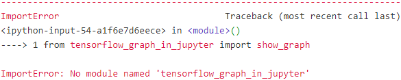
However, I chose another tool - "tfgraphviz"
# At first, we have to install graphviz by using pip install graphviz and pip install tfgraphviz
#################
Previous steps were following introduction on the website"https://pypi.org/project/tfgraphviz/", OR "https://github.com/akimach/tfgraphviz"
but on windows, these steps are not complete
import tfgraphviz as tfg
tfg.board(tf.get_default_graph()).view()
ExecutableNotFound: failed to execute ['dot', '-Tpdf', '-O', 'G.gv'], make sure the Graphviz executables are on your systems' PATH

#################
https://blog.csdn.net/Linli522362242/article/details/104542381
#so, go to website "https://graphviz.gitlab.io/_pages/Download/Download_windows.html"
to download .msi file, and install it and write down the directory where you install it 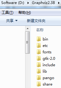
# next step, we have to append it to system environment path

#On jupyter notebook, you have to append the following codes:
import os
os.environ["PATH"] += os.pathsep + "D:/Graphviz2.38/bin" # " directory" where you intall graphviz
# use the following code to test it in Jupyter notebook
import tensorflow as tf
import tfgraphviz as tfg
a = tf.constant(1, name="a")
b = tf.constant(2, name="b")
c = tf.add(a, b, name="add")
g = tfg.board(tf.get_default_graph())
g.view()![]()

Then, Please close "G.gv.pdf" file
Finally,
import tfgraphviz as tfg
tfg.board(tf.get_default_graph()).view()![]()

the following code from https://blog.csdn.net/Linli522362242/article/details/106290394
tf.reset_default_graph()

n_epochs = 1000
learning_rate = 0.01

X = tf.constant( scaled_housing_data_plus_bias, dtype=tf.float32, name="X" ) # X node
y = tf.constant( housing.target.reshape(-1,1), dtype=tf.float32, name="y" )  # y node
                     #random_uniform node
theta = tf.Variable( tf.random_uniform([n+1, 1], -1.0, 1.0, seed=42 ), name="theta" ) # theta node
y_pred = tf.matmul(X, theta, name="predictions")                             # predictions node
error = y_pred-y                                                             #sub node
                     # Square node   #for (y_pred-y)**2 (Const int 2 node)
mse = tf.reduce_mean( tf.square(error), name="mse" )                        # mse node
#GradientDescent: Next theta=current theta - learning_rate * gradients
optimizer = tf.train.GradientDescentOptimizer( learning_rate=learning_rate ) # GradientDescent node
training_op = optimizer.minimize(mse) # 2/m * X^T * (y_pred - y)             # gradients node:
init = tf.global_variables_initializer()                                    #init node
# Just create a Saver node at the end of the construction phase (after all "variable nodes" are created)
saver = tf.train.Saver() ###############Saver##############                #save node

with tf.Session() as sess:
    sess.run(init)

    for epoch in range(n_epochs):
        if epoch%100 ==0: # checkpoint every 100 epochs
            print( "Epoch", epoch, "MSE=", mse.eval() )
            save_path = saver.save(sess, "/tmp/my_model.ckpt") #passing it the session and path of the checkpoint file:
        sess.run(training_op)

    best_theta = theta.eval()
    save_path = saver.save(sess, "/tmp/my_model_final.ckpt")
The first step is to tweak your program a bit so it writes the graph definition and some training stats—for example, the training error (MSE)—to a log directory that TensorBoard will read from. You need to use a different log directory every time you run your program, or else TensorBoard will merge stats from different runs, which will mess up搞乱 the visualizations. The simplest solution for this is to include a timestamp in the log directory name. Add the following code at the beginning of the program:
tf.reset_default_graph()

from datetime import datetime

# utcnow = datetime.utcnow().strftime("%Y/%m/%d %H:%M:%S") #  "2020/05/25 13:31:12"
utcnow = datetime.utcnow().strftime("%Y%m%d%H%M%S") #  "20200525182423"
# print("Current Greenwich Mean Time: ",utcnow)
# nynow = datetime.now().strftime("%Y/%m/%d %H:%M:%S")    #  "2020/05/25 09:31:12"
# print("Current NewYork time: ", nynow)
root_logdir = "tf_logs"
log_dir = "{}/run-{}/".format(root_logdir, utcnow) #'tf_logs/run-2020/05/25 13:31:12/'
#print(log_dir) #tf_logs/run-20200525182423/
n_epochs = 1000
learning_rate = 0.01
X = tf.placeholder( tf.float32, shape=(None, n+1), name="X" ) # X node
y = tf.placeholder( tf.float32, shape=(None, 1), name="y" ) # y node
#Hidden: random_uniform node
theta = tf.Variable( tf.random_uniform([n+1, 1], -1.0, 1.0, seed=42), name="theta") # theta node
y_pred = tf.matmul( X, theta, name="predictions" ) # prediction node
error = y_pred-y # sub node
# Square node and Const (int 2) node
mse = tf.reduce_mean( tf.square(error), name="mse" ) # mse node
optimizer = tf.train.GradientDescentOptimizer( learning_rate=learning_rate )#Gradient Descent node~substructure
training_op = optimizer.minimize(mse) # 2/m * X^T * (y_pred - y) # gradients node ~ substructure
init = tf.global_variables_initializer() #int nodeNext, add the following code at the very end of the construction phase:
# create a node in the graph that will evaluate the MSE value and
# write it to a TensorBoard-compatible binary log string called a summary.
# tf.summary.scalar(tags, values, collections=None, name=None)
mse_summary = tf.summary.scalar("MSE", mse)
# creates a FileWriter that you will use to write summaries to logfiles in the log directory.
# tf.summary.FileWritter(path,sess.graph)
file_writer = tf.summary.FileWriter(log_dir, tf.get_default_graph())
The first line creates a node in the graph that will evaluate the MSE value and write it to a TensorBoard-compatible binary log string called a summary. The second line creates a FileWriter that you will use to write summaries to logfiles in the log directory. The first parameter indicates the path of the log directory (in this case something like "tf_logs/run-20200525182423/", relative to the current directory). The second (optional) parameter is the graph you want to visualize. Upon creation, the File Writer creates the log directory if it does not already exist (and its parent directories
if needed), and writes the graph definition in a binary logfile called an events file.
###################################
WARNING
Avoid logging training stats at every single training step, as this would significantly slow down training.
###################################
n_epochs = 10
batch_size = 100
n_batches = int (np.ceil(m/batch_size) ) #207

def fetch_batch( epoch, batch_index, batch_size ):
    np.random.seed( epoch*n_batches + batch_index )
    indices = np.random.randint(m,size=batch_size)
    X_batch = scaled_housing_data_plus_bias[indices]
    y_batch = housing.target.reshape(-1,1) [indices]
    return X_batch, y_batch

with tf.Session() as sess:
    sess.run(init)

    for epoch in range( n_epochs ):
        for batch_index in range( n_batches ):
            X_batch, y_batch = fetch_batch(epoch, batch_index, batch_size)
            # evaluate the mse_summary node regularly during training (e.g., every 10 mini-batches).
            if batch_index % 10 ==0:
                summary_str = mse_summary.eval( feed_dict={X: X_batch, y: y_batch})
                ## epoch = step/n_batches  and batch_index =step % n_batches
                step = epoch * n_batches + batch_index
                file_writer.add_summary(summary_str, step) # add_summary(y_axis,x_axis)
            sess.run( training_op, feed_dict={X: X_batch, y: y_batch})

    best_theta = theta.eval()
Finally, you want to close the FileWriter at the end of the program:
file_writer.close()

best_theta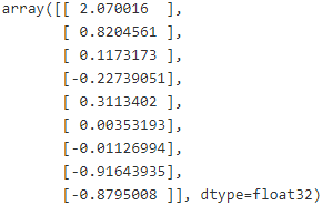
![]()

############################
https://blog.csdn.net/Linli522362242/article/details/104542381
#so, go to website "https://graphviz.gitlab.io/_pages/Download/Download_windows.html"
to download .msi file, and install it and write down the directory where you install it
# next step, we have to append it to system environment path
#On jupyter notebook, you have to append the following codes:
import os
os.environ["PATH"] += os.pathsep + "D:/Graphviz2.38/bin" # " directory" where you intall graphviz
############################
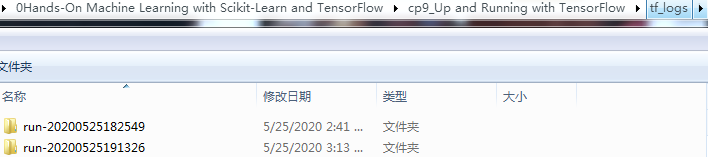
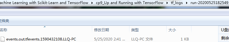
Now run this program: it will create the log directory and write an events file in this directory, containing both the graph definition and the MSE values. Open up a shell and go to your working directory, then type ls -l tf_logs/run* to list the contents of the log directory:
go to:
C:\Users\LlQ\0Hands-On Machine Learning with Scikit-Learn and TensorFlow\cp9_Up and Running with TensorFlow

Next type: "cd.."![]()
Great! Now it's time to fire up the TensorBoard server. You need to activate your virtualenv environment if you created one, then start the server by running the tensor board command, pointing it to the root log directory. This starts the TensorBoard web server, listening on port 6006 (which is “goog” written upside down):
Then type: "tensorboard --logdir=./tf_logs"
Finally: start your web browser and type "http://LlQ-pc:6006"
Next open a browser and go to http://0.0.0.0:6006/ (or http://localhost:6006/). Welcome to TensorBoard! In the Events tab you should see MSE on the right. If you click on it, you will see a plot of the MSE during training, for both runs (Figure 9-3). You can check or uncheck the runs you want to see, zoom in or out, hover over the curve to get details, and so on.
Now click on the Graphs tab. You should see the graph shown in Figure 9-4.
for example: Run: run-20200520200030
Figure 9-4. Visualizing the graph using TensorBoard
VS
To reduce clutter, the nodes that have many edges (i.e., connections to other nodes) are separated out to an auxiliary附加的 area on the right (you can move a node back and forth between the main graph and the auxiliary area by right-clicking on it). Some parts of the graph are also collapsed by default. For example, try hovering over the gradients node, then click on the ⊕ icon to expand this subgraph. Next, in this subgraph, try expanding the mse_grad subgraph.
###################
TIP
If you want to take a peek at the graph directly within Jupyter, you can use the show_graph() function available in the notebook for this chapter. It was originally written by A. Mordvintsev in his great deepdream tutorial notebook. Another option is to install E. Jang's TensorFlow debugger tool which includes a Jupyter extension for graph visualization (and more).
###################
Name Scopes
When dealing with more complex models such as neural networks, the graph can easily become cluttered with thousands of nodes. To avoid this, you can create name scopes to group related nodes. For example, let's modify the previous code to define the error and mse ops within a name scope called "loss":
tf.reset_default_graph()

utcnow = datetime.utcnow().strftime("%Y%m%d%H%M%S")
root_logdir = "tf_logs"
logdir = "{}/run-{}/".format(root_logdir, utcnow)

n_epochs = 1000
learning_rate = 0.01                         #dimension
X = tf.placeholder( tf.float32, shape=(None, n+1), name="X")
y = tf.placeholder( tf.float32, shape=(None, 1), name="y")
theta = tf.Variable(tf.random_uniform([n+1, 1], -1.0, 1.0, seed=42), name="theta")
y_pred = tf.matmul(X, theta, name="predictions")
with tf.name_scope("loss") as scope:
error = y_pred -y
mse = tf.reduce_mean( tf.square(error), name="mse")optimizer = tf.train.GradientDescentOptimizer( learning_rate=learning_rate )
training_op = optimizer.minimize(mse)
init = tf.global_variables_initializer()
mse_summary = tf.summary.scalar("MSE", mse)
file_writer = tf.summary.FileWriter(logdir, tf.get_default_graph() )
n_epochs =10
batch_size = 100
n_batches = int(np.ceil(m/batch_size))
with tf.Session() as sess:
sess.run(init)
for epoch in range(n_epochs):
for batch_index in range( n_batches ):
X_batch, y_batch = fetch_batch(epoch, batch_index, batch_size)
if batch_index %10==0:
summary_str = mse_summary.eval( feed_dict = {X: X_batch, y: y_batch})
# epoch = step/n_batches and batch_index =step % n_batches
step = epoch * n_batches + batch_index
file_writer.add_summary( summary_str, step )
sess.run(training_op, feed_dict={X:X_batch, y: y_batch} )
best_theta = theta.eval()
file_writer.flush()
file_writer.close()
print("Best theta: ")
print(best_theta)
The name of each op defined within the scope is now prefixed with "loss/":
print( error.op.name ) ![]()
print(mse.op.name)![]()
In TensorBoard, the mse and error nodes now appear inside the loss namespace, which appears collapsed by default (Figure 9-5).
click reload this page button  --> choose the new graph
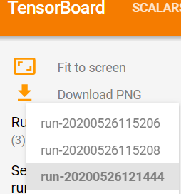
 vs
vs 

Figure 9-5. A collapsed namescope in TensorBoard
tf.reset_default_graph()

a1 = tf.Variable(0, name="a")      # name == "a"
a2 = tf.Variable(0, name="a")      # name == "a_1"

with tf.name_scope( "param" ):     # name == "param"
    a3 = tf.Variable(0, name="a")  # name == "param/a"

with tf.name_scope( "param" ):     # name == "param_1"
    a4 = tf.Variable(0, name="a")  # name == "param_1/a"

for node in (a1, a2, a3, a4) :
print(node.op.name) 
Modularity
Suppose you want to create a graph that adds the output of two rectified矫正的 linear units (ReLU). A ReLU computes a linear function of the inputs, and outputs the result if it is positive, and 0 otherwise, as shown in Equation 9-1.
Equation 9-1. Rectified linear unit![]()
The following code does the job, but it's quite repetitive:
tf.reset_default_graph()

n_features = 3
X = tf.placeholder( tf.float32, shape=(None, n_features), name="X" )

w1 = tf.Variable( tf.random_normal( (n_features,1) ), name="weights1" )
w2 = tf.Variable( tf.random_normal( (n_features,1) ), name="weights2" )
b1 = tf.Variable( 0.0, name="bias1" )
b2 = tf.Variable( 0.0, name="bias2" )

z1 = tf.add( tf.matmul(X, w1), b1, name="z1" ) #prediction
z2 = tf.add( tf.matmul(X, w2), b2, name="z2" )

relu1 = tf.maximum( z1, 0., name="relu1" )
relu2 = tf.maximum( z1, 0., name="relu2" ) # Oops, cut&paste error! Did you spot it? # z1 --> z2

output = tf.add(relu1, relu2, name="output")
Such repetitive code is hard to maintain and error-prone (in fact, this code contains a cut-and-paste error; did you spot it?). It would become even worse if you wanted to add a few more ReLUs. Fortunately, TensorFlow lets you stay DRY (Don't Repeat Yourself): simply create a function to build a ReLU. The following code creates five ReLUs and outputs their sum (note that add_n() creates an operation that will compute the sum of a list of tensors):
tf.reset_default_graph()

def relu(X):
    w_shape = ( int(X.get_shape()[1]), 1 ) # X.get_shape()[1]==features
    w = tf.Variable( tf.random_normal(w_shape), name="weights" ) # ( features, 1 )
    b = tf.Variable( 0.0, name="bias" )
    z = tf.add( tf.matmul(X,w), b, name="z" )
    return tf.maximum( z, 0., name="relu" )

n_features = 3
X = tf.placeholder( tf.float32, shape=(None, n_features), name="X" )
relus = [ relu(X) for i in range(5) ]
output = tf.add_n( relus, name="Output" ) # compute the sum of a list of tensors
Note that when you create a node, TensorFlow checks whether its name already exists, and if it does it appends an underscore followed by an index to make the name unique. So the first ReLU contains nodes named "weights", "bias", "z", and "relu" (plus many more nodes with their default name, such as "MatMul"); the second ReLU contains nodes named "weights_1", "bias_1", and so on; the third ReLU contains nodes named "weights_2", "bias_2", and so on. TensorBoard identifies such series and collapses them together to reduce clutter (as you can see in Figure 9-6).
Figure 9-6. Collapsed node series
Using name scopes, you can make the graph much clearer. Simply move all the content of the relu() function inside a name scope. Figure 9-7 shows the resulting graph. Notice that TensorFlow also gives the name scopes unique names by appending _1, _2, and so on.
tf.reset_default_graph()

def relu(X):
    with tf.name_scope("relu"):               ##############
        w_shape = ( int(X.get_shape()[1]), 1 )
        w = tf.Variable( tf.random_normal(w_shape), name="weights" )
        b = tf.Variable( 0.0, name="bias" )
        z = tf.add( tf.matmul(X, w), b, name="z" )
        return tf.maximum( z, 0., name="max" )##############

X = tf.placeholder( tf.float32, shape=(None, n_features), name="X" )
relus = [ relu(X) for i in range(5) ]
output = tf.add_n( relus, name="output" )

file_writer = tf.summary.FileWriter( "logs/relu2", tf.get_default_graph() )

file_writer.flush()
file_writer.close()
Figure 9-7. A clearer graph using name-scoped units

Sharing Variables
If you want to share a variable between various components of your graph, one simple option is to create it first, then pass it as a parameter to the functions that need it.
For example, suppose you want to control the ReLU threshold (currently hardcoded to 0) using a shared threshold variable for all ReLUs. You could just create that variable first, and then pass it to the relu() function:
tf.reset_default_graph()

def relu( X, threshold ):
    with tf.name_scope( "relu" ): #rectified linear units
        w_shape = ( int(X.get_shape()[1]), 1 )
        w = tf.Variable( tf.random_normal(w_shape), name="weights" )
        b = tf.Variable( 0.0, name="bias" )
        z = tf.add( tf.matmul(X,w), b, name="z" )
        return tf.maximum( z, threshold, name="max" )

threshold = tf.Variable(0.0, name="threshold")
X = tf.placeholder( tf.float32, shape=(None, n_features), name="X" )
relus = [ relu(X, threshold) for i in range(5) ]
output = tf.add_n( relus, name="output" )
This works fine: now you can control the threshold for all ReLUs using the threshold variable. However, if there are many shared parameters such as this one, it will be painful to have to pass them around as parameters all the time. Many people create a Python dictionary containing all the variables in their model, and pass it around to every function. Others create a class for each module (e.g., a ReLU class using class variables to handle the shared parameter). Yet another option is to set the shared variable as an attribute of the relu() function upon the first call, like so: ####################################################################################
tf.reset_default_graph()

def relu(X):
    with tf.name_scope("relu"): #set the shared variable as an attribute of the relu() function upon the first call
        if not hasattr( relu, "threshold"):
            relu.threshold = tf.Variable( 0.0, name="threshold" )
        w_shape = ( int(X.get_shape()[1]), 1)
        w = tf.Variable( tf.random_normal(w_shape), name="weights" )
        b = tf.Variable( 0.0, name="bias" )
        z = tf.add( tf.matmul(X,w), b, name="z")
        return tf.maximum( z, relu.threshold, name="max" )

X = tf.placeholder( tf.float32, shape=(None, n_features), name="X" )
relus = [ relu(X) for i in range(5) ]
output = tf.add_n( relus, name="output" ) 
####################################################################################
TensorFlow offers another option, which may lead to slightly cleaner and more modular code than the previous solutions. This solution is a bit tricky to understand at first, but since it is used a lot in TensorFlow it is worth going into a bit of detail. The idea is to use the get_variable() function to create the shared variable if it does not exist yet, or reuse it if it already exists. The desired behavior (creating or reusing) is controlled by an attribute of the current variable_scope(). ###########################################
For example, the following code will create a variable named "relu/threshold" (as a scalar, since shape=(), and using 0.0 as the initial value):
tf.reset_default_graph()

with tf.variable_scope("relu"):
    threshold = tf.get_variable( "threshold", shape=(), initializer=tf.constant_initializer(0.0) )
Note that if the variable has already been created by an earlier call to get_variable(), this code will raise an exception. This behavior prevents reusing variables by mistake.
If you want to reuse a variable, you need to explicitly say so by setting the variable scope's reuse attribute to True (in which case you don't have to specify the shape or the initializer):
with tf.variable_scope("relu", reuse=True):
    threshold = tf.get_variable("threshold")
This code will fetch the existing "relu/threshold" variable, or raise an exception if it does not exist or if it was not created using get_variable(). Alternatively, you can set the reuse attribute to True inside the block by calling the scope's reuse_variables() method:
with tf.variable_scope("relu") as scope:
    scope.reuse_variables() ############
    threshold = tf.get_variable("threshold")
#############################
WARNING
Once reuse is set to True, it cannot be set back to False within the block. Moreover, if you define other variable scopes inside this one, they will automatically inherit reuse=True. Lastly, only variables created by get_variable() can be reused this way.
#############################
Now you have all the pieces you need to make the relu() function access the threshold variable without having to pass it as a parameter:
tf.reset_default_graph()

def relu(X): # defines the relu() function
    #The desired behavior (creating or reusing) is controlled by an attribute of the current variable_scope()
    with tf.variable_scope("relu", reuse=True):#create name scopes("variable_scope") to group related nodes
        w_shape = int( X.get_shape()[1] ), 1
        w = tf.Variable( tf.random_normal(w_shape), name="weights" )
        b = tf.Variable( 0.0, name="bias" )
        z = tf.add( tf.matmul(X,w), b, name="z" )
        return tf.maximum( z, threshold, name='max' )

X = tf.placeholder( tf.float32, shape=(None, n_features), name="X" )
# create a variable named "relu/threshold" (as a scalar, since shape=(), and using 0.0 as the initial value)
with tf.variable_scope("relu"):
    threshold = tf.get_variable( "threshold", shape=(), initializer=tf.constant_initializer(0.0) ) # relu/threshold
relus = [ relu(X) for relu_index in range(5) ] # relu_#
output = tf.add_n( relus, name="output" )

file_writer = tf.summary.FileWriter( "logs/relu6", tf.get_default_graph() )
file_writer.close()
This code first defines the relu() function, then creates the relu/threshold variable (as a scalar since shape=() that will later be initialized to 0.0) and builds five ReLUs by calling the relu() function. The relu() function reuses the relu/threshold variable, and creates the other ReLU nodes.
Figure 9-8. Five ReLUs sharing the threshold variable
###############################
NOTE
Variables created using get_variable() are always named using the name of their variable_scope as a prefix (e.g.,
"relu/threshold"), but for all other nodes (including variables created with tf.Variable()) the variable scope acts like a new name scope. In particular, if a name scope with an identical name was already created, then a suffix is added to make the name unique. For example, all nodes created in the preceding code (except the threshold variable) have a name prefixed with "relu_1/" to "relu_5/", as shown in Figure 9-8.
###############################
It is somewhat unfortunate that the threshold variable must be defined outside the relu() function, where all the rest of the ReLU code resides. ![]()
![]()
![]()
To fix this, the following code creates the threshold variable within the relu() function upon the first call, then reuses it in subsequent calls. Now the relu() function does not have to worry about name scopes or variable sharing: it just calls get_variable(), which will create or reuse the threshold variable (it does not need to know which is the case). The rest of the code calls relu() five times, making sure to set reuse=False on the first call, and reuse=True
for the other calls.
tf.reset_default_graph()

def relu(X):
    with tf.variable_scope("relu"):
        threshold = tf.get_variable( "threshold", shape=(), initializer=tf.constant_initializer(0.0) )######
        w_shape = (int(X.get_shape()[1]), 1)
        w = tf.Variable( tf.random_normal(w_shape), name="weights" )
        b = tf.Variable( 0.0, name="bias" )
        z = tf.add( tf.matmul(X, w), b, name="z" )
        return tf.maximum( z, threshold, name="max" )

X = tf.placeholder( tf.float32, shape=(None, n_features), name="X" )
with tf.variable_scope("", default_name="") as scope: ###################
    first_relu = relu(X)    #create the shared variable #making sure to set reuse=False on the first call
    scope.reuse_variables() # then reuse
    relus = [first_relu] + [ relu(X) for i in range(4) ]

output = tf.add_n( relus, name="output")

file_writer = tf.summary.FileWriter( "logs/relu8", tf.get_default_graph() )
file_writer.close()

![]()
![]()
![]()
OR
tf.reset_default_graph()

def relu(X):
    threshold = tf.get_variable( "threshold", shape=(), initializer=tf.constant_initializer(0.0) )######
    w_shape = (int(X.get_shape()[1]), 1)
    w = tf.Variable( tf.random_normal(w_shape), name="weights" )
    b = tf.Variable( 0.0, name="bias" )
    z = tf.add( tf.matmul(X, w), b, name="z" )
    return tf.maximum( z, threshold, name="max" )

X = tf.placeholder( tf.float32, shape=(None, n_features), name="X" )

relus = []
for relu_index in range(5):
    with tf.variable_scope("relu", reuse=( relu_index>=1 ) ) as scope: #making sure to set reuse=False on the first call
        relus.append( relu(X))

output = tf.add_n( relus, name="output")

file_writer = tf.summary.FileWriter( "logs/relu9", tf.get_default_graph() )
file_writer.close()
The resulting graph is slightly different than before, since the shared variable lives within the first ReLU(see Figure 9-9).
Figure 9-9. Five ReLUs sharing the threshold variable
![]()
![]()
![]()
This concludes this introduction to TensorFlow. We will discuss more advanced topics as we go through the following chapters, in particular many operations related to deep neural networks深层神经网络, convolutional neural networks卷积神经网络, and recurrent neural networks递归神经网络 as well as how to scale up with TensorFlow using multithreading, queues, multiple GPUs, and multiple servers.
Extra material
tf.reset_default_graph()

with tf.variable_scope("my_scope"): #create name scopes to group related nodes
    # x0: my_scope/x  #get_variable() : create or reuse the threshold variable
    x0 = tf.get_variable( "x", shape=(), initializer=tf.constant_initializer(0.) )
    x1 = tf.Variable(0., name="x") # x1: my_scope/x_1
    x2 = tf.Variable(0., name="x") # x2: my_scope/x_2

with tf.variable_scope("my_scope", reuse=True):
    # get_variable() : create or reuse the threshold variable
    x3 = tf.get_variable("x")      # x3: my_scope/x # x0 is x3 since reuse=True
    x4 = tf.Variable(0., name="x") # my_score_1/x
    #since it's a separate block from the first one, the name of the scope is made unique by TensorFlow
    #(my_scope_1) and thus the variable x4 is named my_scope_1/x

with tf.variable_scope("", default_name="", reuse=True):
    x5 = tf.get_variable("my_scope/x")


print("x0:", x0.op.name)
print("x1:", x1.op.name)
print("x2:", x2.op.name)

print("x3:", x3.op.name)
print("x4:", x4.op.name)

print("x5:", x5.op.name)

print(x0 is x3 and x3 is x5) 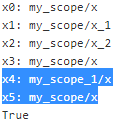
The first variable_scope() block first creates the shared variable x0(tf.get_variable( "x", shape=(), initializer=tf.constant_initializer(0.) )), named my_scope/x. For all operations other than shared variables (including non-shared variables), the variable scope acts like a regular name scope(create name scopes to group related nodes), which is why the two variables x1 and x2 have a name with a prefix my_scope/. Note however that TensorFlow makes their names unique by adding an index: my_scope/x_1 and my_scope/x_2.
The second variable_scope() block reuses the shared variables in scope my_scope, which is why x0 is x3. Once again, for all operations other than shared variables it acts as a named scope, and since it's a separate block( with tf.variable_scope("my_scope", reuse=True): ...) from the first one(with tf.variable_scope("my_scope"): ...), the name of the scope is made unique by TensorFlow (my_scope_1) and thus the variable x4 is named my_scope_1/x.
The third block shows another way to get a handle on the shared variable my_scope/x by creating a variable_scope() at the root scope (whose name is an empty string), then calling get_variable() with the full name of the shared variable (i.e. "my_scope/x").
Exercise
- What are the main benefits of creating a computation graph rather than directly executing the computations? What are the main drawbacks?
Main benefits and drawbacks of creating a computation graph rather than directly executing the computations:
• Main benefits:
—TensorFlow can automatically compute the gradients for you (using reverse-mode autodiff).
—TensorFlow can take care of running the operations in parallel in different threads.
—It makes it easier to run the same model across different devices.
—It simplifies introspection内省—for example, to view the model in TensorBoard.
• Main drawbacks:
—It makes the learning curve steeper陡峭的.
—It makes step-by-step debugging harder.
- Is the statement a_val = a.eval(session=sess) equivalent to a_val = sess.run(a)?
Yes, the statement a_val = a.eval(session=sess) is indeed equivalent to a_val = sess.run(a).x = tf.Variable(3, name='x') y = tf.Variable(4, name='y') f = x*x*y+y+2 with tf.Session() as sess: # the session is set as the default session x.initializer.run() #==tf.get_default_session().run(x.initializer) y.initializer.run() result = f.eval() #==tf.get_default_session().run(f) #the session is automatically closed at the end of the block result # 42OR
sess = tf.Session() #creates a session sess.run(x.initializer) #initializes the variables sess.run(y.initializer) result = sess.run(f) #evaluates f # 42 sess.close() # closes the session (which frees up resources) - Is the statement a_val, b_val = a.eval(session=sess), b.eval(session=sess) equivalent to a_val, b_val = sess.run([a, b])?
No, the statement a_val, b_val = a.eval(session=sess), b.eval(session=sess) is not equivalent to a_val, b_val = sess.run([a, b]). Indeed, the first statement runs the graph twice (once to compute a, once to compute b), while the second statement runs the graph only once. If any of these operations (or the ops they depend on) have side effects (e.g., a variable is modified, an item is inserted in a queue, or a reader reads a file), then the effects will be different. If they don't have side effects, both statements will return the same result, but the second statement will be faster than the first.# First, this code defines a very simple graph. w = tf.constant(3) #tf.constant(3): Creates a constant tensor x = w + 2 y = x + 5 z = x * 3 # Then it starts a session and runs the graph to evaluate with tf.Session() as sess: print(y.eval()) # 10 # runs the graph(containing nodes[w,x,y,z]) to evaluate y # first evaluates w, then x, then y; print(z.eval()) # 15 # Finally, the code runs the graph to evaluate zwith tf.Session() as sess: y_val, z_val = sess.run([y,z]) # evaluate both y and z in just one graph run print(y_val) # 10 print(z_val) # 15 - Can you run two graphs in the same session?
No, you cannot run two graphs in the same session. You would have to merge the graphs into a single graph first.
- If you create a graph g containing a variable w, then start two threads and open a session in each thread, both using the same graph g, will each session have its own copy of the variable w or will it be shared?
In local TensorFlow, sessions manage variable values, so if you create a graph g containing a variable w, then start two threads and open a local session in each thread, both using the same graph g, then each session will have its own copy of the variable w.
However, in distributed TensorFlow, variable values are stored in containers managed by the cluster, so if both sessions connect to the same cluster and use the same container, then they will share the same variable value for w.
- When is a variable initialized? When is it destroyed?
A variable is initialized when you call its initializer, and it is destroyed when the session ends. In distributed TensorFlow, variables live in containers on the cluster, so closing a session will not destroy the variable. To destroy a variable, you need to clear its container.
- What is the difference between a placeholder and a variable?
Variables and placeholders are extremely different, but beginners often confuse them:
• A variable is an operation that holds a value. If you run the variable, it returns that value. Before you can run it, you need to initialize it. You can change the variable's value (for example, by using an assignment operation). It is stateful: the variable keeps the same value upon successive runs of the graph. It is typically used to hold model parameters but also for other purposes (e.g., to count the global training step).
• Placeholders technically don't do much: they just hold information about the type and shape of the tensor they represent, but they have no value. In fact, if you try to evaluate an operation that depends on a placeholder, you must feed TensorFlow the value of the placeholder (using the feed_dict argument) or else you will get an exception. Placeholders are typically used to feed training or test data to TensorFlow during the execution phase. They are also useful to pass a value to an assignment node, to change the value of a variable (e.g., model weights).n_epochs = 1000 learning_rate = 0.01 tf.reset_default_graph() X = tf.placeholder( tf.float32, shape=(None, n+1), name="X" ) ###### y = tf.placeholder( tf.float32, shape=(None, 1), name="y" ) ###### theta = tf.Variable( tf.random_uniform([n+1, 1], -1.0, 1.0, seed=42), name="theta" ) y_pred = tf.matmul( X, theta, name="prediction" ) error = y_pred - y mse = tf.reduce_mean( tf.square(error), name="mse" ) optimizer = tf.train.GradientDescentOptimizer( learning_rate = learning_rate ) training_op = optimizer.minimize(mse) init = tf.global_variables_initializer() n_epochs = 10 batch_size = 100 n_batches = int(np.ceil( housing.data.shape[0]/batch_size )) #housing.data.shape[0]: the number of samples def fetch_batch( epoch, batch_index, batch_size ): np.random.seed( epoch*n_batches + batch_index ) indices = np.random.randint(m,size=batch_size) X_batch = scaled_housing_data_plus_bias[indices] y_batch = housing.target.reshape(-1,1) [indices] return X_batch, y_batch with tf.Session() as sess: sess.run(init) # execution for epoch in range(n_epochs): for batch_index in range(n_batches): X_batch, y_batch = fetch_batch( epoch, batch_index, batch_size ) sess.run( training_op, feed_dict={X: X_batch, y: y_batch}) #feed best_theta = theta.eval() best_thetahttps://blog.csdn.net/Linli522362242/article/details/106290394
- What happens when you run the graph to evaluate an operation that depends on a placeholder but you don't feed its value? What happens if the operation does not depend on the placeholder?
If you run the graph to evaluate an operation that depends on a placeholder but you don't feed its value, you get an exception. If the operation does not depend on the placeholder, then no exception is raised.
- When you run a graph, can you feed the output value of any operation, or just the value of placeholders?
When you run a graph, you can feed the output value of any operation, not just the value of placeholders. In practice, however, this is rather rare (it can be useful,
for example, when you are caching the output of frozen layers; see Chapter 11).
- How can you set a variable to any value you want (during the execution phase)?
You can specify a variable's initial value when constructing the graph, and it will be initialized later when you run the variable's initializer during the execution phase. If you want to change that variable's value to anything you want during the execution phase, then the simplest option is to create an assignment node (during
the graph construction phase) using the tf.assign() function, passing the variable and a placeholder as parameters. During the execution phase, you can run the assignment operation and feed the variable's new value using the placeholder.import tensorflow as tf x = tf.Variable(tf.random_uniform(shape=(), minval=0.0, maxval=1.0)) x_new_val = tf.placeholder(shape=(), dtype=tf.float32)### x_assign = tf.assign(x, x_new_val)####################### with tf.Session(): x.initializer.run() # random number is sampled *now* print(x.eval()) # 0.646157 (some random number) x_assign.eval(feed_dict={x_new_val: 5.0})############ print(x.eval()) # 5.0 - How many times does reverse-mode autodiff need to traverse the graph in order to compute the gradients of the cost function with regards to 10 variables? What about forward-mode autodiff? And symbolic differentiation?
Reverse-mode autodiff (implemented by TensorFlow) needs to traverse the graph only twice in order to compute the gradients of the cost function with regards to any number of variables.
################################
https://blog.csdn.net/Linli522362242/article/details/106290394
Figure D-3. Reverse-mode autodiff for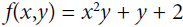 with regards to x at x = 3 and y = 4
Figure D-3 represents the second pass. During the first pass, all the node values were computed, starting from x = 3 and y = 4. You can see those values at the bottom right of each node (e.g.,: x × x =3 × 3= 9,  × y = 9 × 4 = 36, y + 2 = 4 + 2 = 6, 36 + 6 = 42 ). The nodes are labeled n1 to n7 for clarity. The output node is
  : f(3,4) =
  = 42.
= 42.
The idea is to gradually go down the graph, computing the partial derivative of f(x,y) with regards to each consecutive node, until we reach the variable nodes. For this, reverse-mode autodiff relies heavily on the chain rule, shown in Equation D-4.
Equation D-4. Chain rule
Since is the output node, f = so trivially  = 1.
= 1.Let's continue down the graph to
 : how much does f vary when varies? The answer is
  . We already know that
  = 1, so all we need is
  . Since simply performs the sum
  =, we find that
  , so
, so 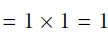 .
.Now we can proceed to node
 : how much does f vary when varies? The answer is
 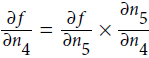 . Since
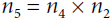 , we find that
  , so
, so  .
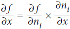
.The process continues until we reach the bottom of the graph. At that point we will have calculated all the partial derivatives of f(x,y) at the point x = 3 and y = 4. In this example, we find ∂f/∂x =
Reverse-mode autodiff requires only one forward pass plus one reverse pass per output to compute all the partial derivatives for all outputs with regards to all the inputs.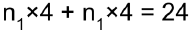 =2xy=2*3*4=24 and ∂f/∂y =
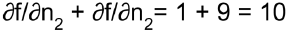 =x^2 +1=3^2 + 1=10 . Sounds about right! ######
################################
On the other hand, forward-mode autodiff would need to run once for each variable (so 10 times if we want the gradients with regards to 10 different variables).
https://blog.csdn.net/Linli522362242/article/details/106290394
################Figure D-2 shows how forward-mode autodiff computes the partial derivative of f(x,y)=
 with regards to x at x = 3 and y = 4. All we need to do is compute f(3 + ϵ, 4); this will output a dual number whose first component is equal to f(3, 4) and whose second component is equal to
  .
.
Figure D-2. Forward-mode autodiff = 0 (but ϵ ≠ 0)
To compute
 =10 we would have to go through the graph again, but this time with x = 3 and y = 4 + ϵ.
So forward-mode autodiff is much more accurate than numerical differentiation, but it suffers from the same major flaw缺点: if there were 1,000 parameters, it would require 1,000 passes through the graph to compute all the partial derivatives. This is where reverse-mode autodiff shines: it can compute all of them in just two passes through the graph.
################
As for symbolic differentiation, it would build a different graph to compute the gradients, so it would not traverse the original graph at all (except when building the new gradients graph). A highly optimized symbolic differentiation system could potentially run the new gradients graph only once to compute the gradients with regards to all variables, but that new graph may be horribly complex and inefficient compared to the original graph.
###########################
https://blog.csdn.net/Linli522362242/article/details/106290394
Symbolic Differentiation符号积分
Figure D-1 shows how symbolic differentiation works on an even simpler function, g(x,y) = 5 + xy. The graph for that function is represented on the left. After symbolic differentiation, we get the graph on the right, which represents the partial derivative = 0 + 0 × x + y × 1 = y (we could similarly obtain the partial derivative with regards to y, ∂g/∂y = x ).
Figure D-1. Symbolic differentiation
In this case, simplification is fairly easy, but for a more complex function, symbolic differentiation can produce a huge graph that may be tough to simplify and lead to suboptimal performance. Most importantly, symbolic differentiation cannot deal with functions defined with arbitrary code—for example, the following function discussed in following:
def my_func(a, b):
    z = 0
    for i in range(100):
    z = a * np.cos(z + i) + z * np.sin(b - i)
return z
###########################
- Implement Logistic Regression with Mini-batch Gradient Descent using TensorFlow. Train it and evaluate it on the moons dataset (introduced in https://blog.csdn.net/Linli522362242/article/details/104151351). Try adding all the bells and whistles:
from sklearn.datasets import make_moons

m=1000
X_moons, y_moons = make_moons(m, noise=0.1, random_state=42)

# Let's take a peek at the dataset:
import matplotlib.pyplot as plt

plt.plot(X_moons[y_moons==1, 0], X_moons[y_moons==1, 1], "go", label="Positive")
plt.plot(X_moons[y_moons==0, 0], X_moons[y_moons==0, 1], "r^", label="Negative")
plt.legend()
plt.show()
We must not forget to add an extra bias feature ( =1) to every instance. For this, we just need to add a column full of 1s on the left of the input matrix
  :
: X_moons_with_bias = np.c_[ np.ones((X_moons.shape[0],1)), X_moons] X_moons_with_bias[:5]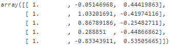 #Looks good.
Now let's reshape y_train to make it a column vector (i.e. a 2D array with a single column):
Now let's split the data into a training set and a test set:y_moons_column_vector = y_moons.reshape(-1,1) # shape: (1000, 1)
Ok, now let's create a small function to generate training batches. In this implementation we will just pick random instances from the training set for each batch. This means that a single batch may contain the same instance multiple times, and also a single epoch may not cover all the training instances (in fact it will generally cover only about two thirds of the instances). However, in practice this is not an issue and it simplifies the code:test_ratio = 0.2 test_size = int(m*test_ratio) X_train = X_moons_with_bias[:-test_size] X_test = X_moons_with_bias[-test_size:] y_train = y_moons_column_vector[:-test_size] y_test = y_moons_column_vector[-test_size:]def random_batch( X_train, y_train, batch_size): rnd_indices = np.random.randint( 0, len(X_train), batch_size ) X_batch = X_train[rnd_indices] y_batch = y_train[rnd_indices] return X_batch, y_batch X_batch, y_batch = random_batch(X_train, y_train, 5) X_batch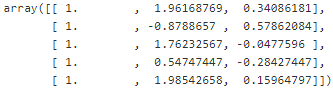
y_batch
Great! Now that the data is ready to be fed to the model, we need to build that model. Let's start with a simple implementation, then we will add all the bells and whistles.
Now let's build the Logistic Regression model. As we saw in# First let's reset the default graph. tf.reset_default_graph() # The moons dataset has "two input features", since each instance is a point on a plane (i.e., 2-Dimensional): n_inputs =2 # X_moons.shape[1]
https://blog.csdn.net/Linli522362242/article/details/104005906, this model first computes a weighted sum of the inputs (just like the Linear Regression model),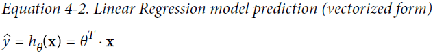
and then it applies the sigmoid function to the result, which gives us the estimated probability for the positive class:
https://blog.csdn.net/Linli522362242/article/details/104070847
Equation 4-13. Logistic Regression model estimated probability (vectorized form)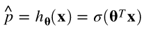
Recall that is the parameter vector, containing the bias term
  and the weights
  . The input vector
  contains a constant term
  , as well as all the input features
  .
.
Since we want to be able to make predictions for multiple instances at a time, we will use an input matrix rather than a single input vector. The
  row will contain the transpose of the
  input vector
  . It is then possible to estimate the probability that each instance belongs to the positive class using the following equation:
 # note each row is an instance
That's all we need to build the model:
In fact, TensorFlow has a nice functionX = tf.placeholder( tf.float32, shape=(None, n_inputs+1), name="X") y = tf.placeholder( tf.float32, shape=(None, 1), name="y") theta = tf.Variable( tf.random_uniform([n_inputs+1, 1], -1.0,1.0, seed=42), name="theta") #one column vector logits = tf.matmul( X, theta, name="logits") y_proba = 1/ ( 1+tf.exp(-logits) )tf.sigmoid()that we can use to simplify the last line of the previous code:
As we saw in (https://blog.csdn.net/Linli522362242/article/details/104070847), the log loss is a good cost function to use for Logistic Regression:y_proba = tf.sigmoid( logits )
Equation 4-16. Cost function of a single training instance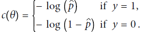 OR
OR 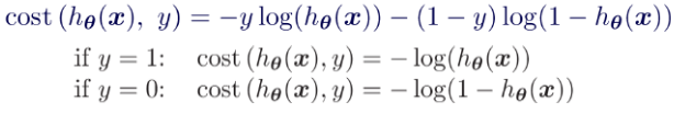
Equation 4-17. Logistic Regression cost function (log loss)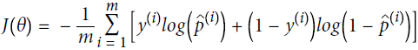
Equation 4-18. Logistic cost function partial derivatives

But we might as well use TensorFlow'sepsilon = 1e-7 # to avoid an overflow when computing the log loss = -tf.reduce_mean( y*tf.log(y_proba + epsilon) + (1-y)*tf.log(1-y_proba + epsilon) )tf.losses.log_loss()function:
The rest is pretty standard: let's create the optimizer and tell it to minimize the cost function:loss = tf.losses.log_loss(y,y_proba) # uses epsilon = 1e-7 by default
All we need now (in this minimal version) is the variable initializer:learning_rate = 0.01 optimizer = tf.train.GradientDescentOptimizer( learning_rate=learning_rate ) training_op = optimizer.minimize(loss)
And we are ready to train the model and use it for predictions!init = tf.global_variables_initializer()
There's really nothing special about this code, it's virtually the same as the one we used earlier for Linear Regression:n_epochs = 1000 batch_size = 50 n_batches = int( np.ceil(m/batch_size) ) with tf.Session() as sess: sess.run(init) for epoch in range(n_epochs): for batch_index in range(n_batches): X_batch, y_batch = random_batch( X_train, y_train, batch_size ) sess.run( training_op, feed_dict = {X: X_batch, y: y_batch} ) # fit or training # loss = -tf.reduce_mean(y * tf.log(y_proba + epsilon) + (1 - y) * tf.log(1 - y_proba + epsilon)) loss_val = loss.eval( {X: X_test, y: y_test} ) #transform base on the result of training if epoch % 100 == 0: print("Epoch: ", epoch, "\tLoss: ", loss_val) # y_proba = 1 / (1 + tf.exp(-logits)) y_proba_val = y_proba.eval( feed_dict={X: X_test, y: y_test} )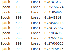
Note: we don't use the epoch number when generating batches, so we could just have a singleforloop rather than 2 nestedforloops, but it's convenient to think of training time in terms of number of epochs (i.e., roughly the number of times the algorithm went through the training set).
For each instance in the test set,y_proba_valcontains the estimated probability that it belongs to the positive class, according to the model. For example, here are the first 5 estimated probabilities:y_proba_val[:5]
To classify each instance, we can go for maximum likelihood: classify as positive any instance whose estimated probability is greater or equal to 0.5:
Equation 4-15. Logistic Regression model prediction https://blog.csdn.net/Linli522362242/article/details/104070847
 y_pred = (y_proba_val >=0.5 ) y_pred[:5]
Depending on the use case, you may want to choose a different threshold than 0.5: make it higher if you want high precision (but lower recall), and make it lower if you want high recall (but lower precision). See https://blog.csdn.net/Linli522362242/article/details/103786116 for more details.
Precision = TP/(TP+FP) # True predicted as Positive/ (True predicted as Positive+ False predicted as Positive)
Recall = TP/(TP+FN) # True predicted as Positive class/ (True predicted as Positive+ False predicted as Negative)
Let's compute the model's precision and recall:from sklearn.metrics import precision_score, recall_score precision_score(y_test, y_pred)
recall_score(y_test, y_pred)
Let's plot these predictions to see what they look like:y_pred_idx = y_pred.reshape(-1) # a 1D array rather than a column vector plt.plot( X_test[y_pred_idx, 1], X_test[y_pred_idx, 2], "yo", label="Positive" ) plt.plot( X_test[~y_pred_idx, 1], X_test[~y_pred_idx,2], "b^", label="Negative") plt.legend() plt.show()
Well, that looks pretty bad, doesn't it? But let's not forget that the Logistic Regression model has a linear decision boundary, so this is actually close to the best we can do with this model (unless we add more features, as we will show in a second).
Now let's start over, but this time we will add all the bells and whistles, as listed in the exercise:
One option is to implement it ourselves:
* Define the graph within a logistic_regression() function that can be reused easily.
* Save checkpoints using a Saver at regular intervals during training, and save the final model at the end of training.
* Restore the last checkpoint upon startup if training was interrupted.
* Define the graph using nice scopes so the graph looks good in TensorBoard.
* Add summaries to visualize the learning curves in TensorBoard.
* Try tweaking some hyperparameters such as the learning rate or the mini-batch size and look at
the shape of the learning curve.
Before we start, we will add 4 more features to the inputs: . This was not part of the exercise, but it will demonstrate how adding features can improve the model. We will do this manually, but you could also add them using
 sklearn.preprocessing.PolynomialFeatures.X_train_enhanced = np.c_[X_train, np.square(X_train[:,1]), np.square(X_train[:,2]), X_train[:,1]**3, X_train[:,2]**3 ] x_train_enhanced = np.c_[X_test, np.square(X_test[:,1]), np.square(X_test[:,2]), X_test[:,1]**3, X_test[:,2]**3 ] # This is what the "enhanced" training set looks like: X_train_enhanced[:3]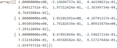
Ok, next let's reset the default graph:
tf.reset_default_graph()Now let's define the
logistic_regression()function to create the graph. We will leave out the definition of the inputsXand the targetsy. We could include them here, but leaving them out will make it easier to use this function in a wide range of use cases (e.g. perhaps we will want to add some preprocessing steps for the inputs before we feed them to the Logistic Regression model).def logistic_regression( X,y, initializer=None, seed=42, learning_rate=0.01 ): n_inputs_including_bias = int(X.get_shape()[1]) #features+bias with tf.name_scope("logistic_regression"): with tf.name_scope("model"): if initializer is None: initializer = tf.random_uniform( [n_inputs_including_bias,1], -1.0, 1.0, seed=seed ) theta = tf.Variable(initializer, name="theta") # X*theta logits = tf.matmul(X, theta, name="logits") # prediction # y_proba = 1/ ( 1+tf.exp(-logits) ) y_proba = tf.sigmoid(logits) with tf.name_scope("train"): # loss = -tf.reduce_mean( y*tf.log(y_proba + epsilon) + (1-y)*tf.log(1-y_proba + epsilon) ) loss = tf.losses.log_loss( y, y_proba, scope="loss" ) optimizer = tf.train.GradientDescentOptimizer( learning_rate=learning_rate ) training_op = optimizer.minimize(loss) loss_summary = tf.summary.scalar('log_loss', loss) #shape=() with tf.name_scope("init"): init = tf.global_variables_initializer() with tf.name_scope("save"): saver = tf.train.Saver() return y_proba, loss, training_op, loss_summary, init, saverLet's create a little function to get the name of the log directory to save the summaries for Tensorboard:
from datetime import datetime

def log_dir( prefix=""):
    now = datetime.utcnow().strftime("%Y%m%d%H%M%S")
    root_logdir = "tf_logs"
    if prefix:
        prefix += "-"
    name = prefix + "run-" + now
    return "{}/{}".format(root_logdir, name)
Next, let's create the graph, using the
logistic_regression()function. We will also create theFileWriterto save the summaries to the log directory for Tensorboard:n_inputs = 2 + 4 logdir = log_dir("logreg") X = tf.placeholder( tf.float32, shape=(None, n_inputs+1), name="X") y = tf.placeholder( tf.float32, shape=(None, 1), name="y" ) y_proba, loss, training_op, loss_summary, init, saver = logistic_regression(X,y) file_writer = tf.summary.FileWriter( logdir, tf.get_default_graph() )

At last we can train the model! We will start by checking whether a previous training session was interrupted, and if so we will load the checkpoint and continue training from the epoch number we saved. In this example we just save the epoch number to a separate file, but in chapter 11 we will see how to store the training step directly as part of the model, using a non-trainable variable calledglobal_stepthat we pass to the optimizer'sminimize()method.
You can try interrupting training to verify that it does indeed restore the last checkpoint when you start it again.import os n_epochs = 10001 batch_size =50 n_batches = int( np.ceil(m/batch_size) ) checkpoint_path = "/tmp/my_logreg_model.ckpt" checkpoint_epoch_path = checkpoint_path + ".epoch" final_model_path = "./my_logreg_model" with tf.Session() as sess: if os.path.isfile(checkpoint_epoch_path): # if the checkpoint file exists, restore the model and load the epoch number with open(checkpoint_epoch_path, "rb") as f: start_epoch = int( f.read() ) print( "Training was interrupted. Continuing at epoch", start_epoch ) saver.restore(sess, checkpoint_path) else: start_epoch = 0 sess.run( init ) for epoch in range(start_epoch, n_epochs ): for batch_index in range(n_batches): X_batch, y_batch = random_batch(X_train_enhanced, y_train, batch_size ) sess.run( training_op, feed_dict={X:X_batch, y:y_batch} ) # fit #loss = -tf.reduce_mean( y*tf.log(y_proba + epsilon) + (1-y)*tf.log(1-y_proba + epsilon) ) #loss = tf.losses.log_loss( y, y_proba, scope="loss" ) #loss_summary = tf.summary.scalar('log_loss', loss) #shape=() loss_val, summary_str = sess.run([loss, loss_summary], feed_dict = {X: X_test_enhanced, y: y_test}) file_writer.add_summary(summary_str, epoch) if epoch % 500 ==0: print("Epoch: ", epoch, "\tLoss:", loss_val) saver.save( sess, checkpoint_path) with open( checkpoint_epoch_path, "wb") as f: f.write( b"%d" % (epoch+1) ) saver.save(sess, final_model_path) y_proba_val = y_proba.eval( feed_dict={X: X_test_enhanced, y: y_test} ) os.remove(checkpoint_epoch_path)run
 --> when you see Epoch: 2500 then click


Once again, we can make predictions by just classifying as positive all the instances whose estimated probability is greater or equal to 0.5:
y_pred = (y_proba_val >=0.5)

precision_score(y_test, y_pred)
recall_score(y_test, y_pred)
y_pred_idx = y_pred.reshape(-1) # a 1D array rather than a column vector
plt.plot( X_test[y_pred_idx, 1], X_test[y_pred_idx,2], "yo", label="Positive" )
plt.plot( X_test[~y_pred_idx, 1], X_test[~y_pred_idx,2], "b^", label="Negative")
plt.legend()
plt.show()
Now that's much, much better! Apparently the new features really helped a lot.
Try starting the tensorboard server, find the latest run and look at the learning curve (i.e., how the loss evaluated on the test set evolves as a function of the epoch number):
tensorboard --logdir=tf_logs

Now you can play around with the hyperparameters (e.g. thebatch_sizeor thelearning_rate) and run training again and again, comparing the learning curves. You can even automate this process by implementing grid search or randomized search. Below is a simple implementation of a randomized search on both the batch size and the learning rate. For the sake of simplicity, the checkpoint mechanism was removed.from scipy.stats import reciprocal n_search_iterations = 10 for search_iteration in range(n_search_iterations): batch_size = np.random.randint(1, 100) #rvs: Random Variates of given type and Size learning_rate = reciprocal(0.0001, 0.1).rvs(random_state=search_iteration) n_inputs = 2+4 logdir = log_dir("logreg") print("Iteration", search_iteration) print(" logdir:", logdir) print(" batch size:", batch_size) print(" learning_rate:", learning_rate) print(" training: ", end="") tf.reset_default_graph() X = tf.placeholder(tf.float32, shape=(None, n_inputs+1), name="X") y = tf.placeholder(tf.float32, shape=(None, 1), name="y") y_proba, loss, training_op, loss_summary, init, saver = logistic_regression( X,y, learning_rate = learning_rate ) file_writer = tf.summary.FileWriter( logdir, tf.get_default_graph() ) n_epochs = 10001 n_batches = int( np.ceil(m/batch_size) ) final_model_path = "./my_logreg_model_%d" % search_iteration with tf.Session() as sess: sess.run(init) for epoch in range(n_epochs): for batch_index in range(n_batches): X_batch, y_batch = random_batch(X_train_enhanced, y_train, batch_size) sess.run( training_op, feed_dict={X: X_batch, y: y_batch} ) loss_val, summary_str = sess.run([loss, loss_summary], feed_dict={X: X_test_enhanced, y:y_test}) file_writer.add_summary(summary_str, epoch) if epoch % 500 ==0: print(".", end="") saver.save( sess, final_model_path ) print() y_proba_val = y_proba.eval( feed_dict={X:X_test_enhanced, y:y_test} ) y_pred = (y_proba_val>0.5) print(" precision:", precision_score(y_test, y_pred)) print(" recall:", recall_score(y_test, y_pred))


Thereciprocal()function from SciPy'sstatsmodule returns a random distribution that is commonly used when you have no idea of the optimal scale of a hyperparameter. See the exercise solutions for https://blog.csdn.net/Linli522362242/article/details/103646927 for more details.
######
the scale of the samples is picked from a uniform distribution within a given range从给定范围内的均匀分布中选取样本的比例(eg.I set reciprocal(150000, 160000)), which is why the right graph, which represents the log of the samples, looks roughly constant. This distribution is useful when you don't have a clue of what the target scale目标比例 is:reciprocal_distrib = reciprocal(20, 200000) #the previous code, I set reciprocal(150000, 160000) #log-uniform distribution samples = reciprocal_distrib.rvs(10000, random_state=42) plt.figure(figsize=(10, 4)) plt.subplot(121) plt.title("Reciprocal distribution (scale=1.0)") plt.hist(samples, bins=50) plt.subplot(122) plt.title("Log of this distribution") plt.hist(np.log(samples), bins=50) plt.show()


 3105
3105


 被折叠的 条评论
为什么被折叠?
被折叠的 条评论
为什么被折叠?
 到【灌水乐园】发言


