


16_NLP stateful CharRNN_window_Tokenizer_stationary_celab_ResetState_character word level_regex_IMDb: https://blog.csdn.net/Linli522362242/article/details/115388298
16_2NLP RNN_colab tensorboard_os.curdir_Pretrained Embed_TrainingSampler_Encoder–Decoder_Greedy Search_Exhaustive Search_Beam search_masking : https://blog.csdn.net/Linli522362242/article/details/115518150
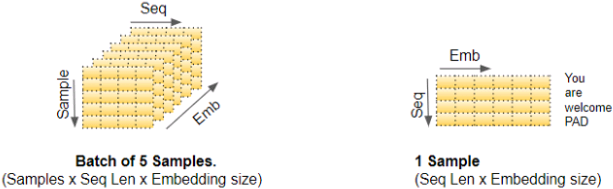
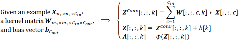
(batch size, number of time steps or sequence length in tokens, d dimentions)
Attention Mechanisms
 Figure 16-3. A simple machine translation model(just sending the encoder’s final hidden state to the decoder)
Consider the path from the word “milk” to its translation “lait” in Figure 16-3: it is quite long! This means that a representation of this word (along with all the other
words) needs to be carried over many steps before it is actually used. Can’t we make this path shorter?(序列中(或者句子中)每个单词的翻译就是一个time step,如果做翻译的时候使用beam search的方法,除了第一个单词外,之后的每个单词的翻译选择都要考虑到最终所有单词的翻译组合能够的最高分(当前这个单词的翻译选择需要在它之后的几个单词的翻译甚至到句子结束<eos>才能确定下来),这说明每个单词翻译之间存在着关联,这里将这种关联直接转化成权重。换句话说,在每个单词翻译的时候,使用权重直接找到能够使得最终所有单词的翻译组合得到最高分的单词翻译)
This was the core idea in a groundbreaking开创性的 2014 paper(Dzmitry Bahdanau et al., “Neural Machine Translation by Jointly Learning to Align and Translate,” arXiv preprint arXiv:1409.0473 (2014).) by Dzmitry Bahdanau et al. They introduced a technique that allowed the decoder to focus on the appropriate words (as encoded by the encoder) at each time step. For example, at the time step where the decoder needs to output the word “lait,” it will focus its attention on the word “milk.” This means that the path from an input word to its translation is now much shorter, so the short-term memory limitations of RNNs have much less impact. Attention mechanisms revolutionized neural machine translation (and NLP in general), allowing a significant improvement in the state of the art, especially for long sentences (over 30 words)(The most common metric used in NMT is the BiLingual Evaluation Understudy (BLEU) score, which compares each translation produced by the model with several good translations produced by humans: it counts the number of n-grams (sequences of n words) that appear in any of the target translations and adjusts the score to take into account the frequency of the produced n-grams in the target translations.).
 Figure 16-6. Neural machine translation using an Encoder–Decoder network with an attention model
Figure 16-6 shows this model’s architecture (slightly simplified, as we will see). On the left, you have the encoder and the decoder. Instead of just sending the encoder’s final hidden state to the decoder (which is still done, although it is not shown in the figure), we now send all of its outputs![]() to the decoder. At each time step, the decoder’s memory cell computes a weighted sum of all these encoder outputs ( the weight
to the decoder. At each time step, the decoder’s memory cell computes a weighted sum of all these encoder outputs ( the weight ![]() OR
OR ![]() is the weight of the
is the weight of the ![]() encoder output
encoder output![]() at the
at the ![]() decoder time step.
decoder time step.![]() ) : this determines which words it will focus(e.g.
) : this determines which words it will focus(e.g.![]() =0) on at this step. For example, if the weight
=0) on at this step. For example, if the weight ![]() is much larger than the weights
is much larger than the weights ![]() and
and![]() , then the decoder will pay much more attention to word number 2 (“milk”) than to the other two words, at least at this time step.
, then the decoder will pay much more attention to word number 2 (“milk”) than to the other two words, at least at this time step.
![]() is the alignment score vector. The decoder decides which part of the source sentence it needs to pay attention to, instead of having encoder encode all the information of the source sentence into a fixed-length vector.
is the alignment score vector. The decoder decides which part of the source sentence it needs to pay attention to, instead of having encoder encode all the information of the source sentence into a fixed-length vector.
![]() is the attention weight vector (=the number of time steps in encoder output) at the
is the attention weight vector (=the number of time steps in encoder output) at the ![]() decoder time step. We apply a softmax activation function to the alignment scores to obtain the attention weights.
decoder time step. We apply a softmax activation function to the alignment scores to obtain the attention weights.
![]() is the attention Context Vector(=1x the number units in LSTMcell/GRUcell) at the the
is the attention Context Vector(=1x the number units in LSTMcell/GRUcell) at the the ![]() decoder time step.
decoder time step.
The rest of the decoder works just like earlier: at each time step the memory cell
- receives the inputs
(###
all these encoder outputs( is from 1 to n), e.g. at the
  decoder time step,

 and where x is the query <==at the time step
 <== a key
  that is closer to the given query
  will get more attention via a larger attention weight
 assigned to the key’s corresponding value
  .
.
###) we just discussed, ###.(序列中(或者句子中)每个单词的翻译就是一个time step,如果做翻译的时候使用beam search的方法,除了第一个单词外,之后的每个单词的翻译选择都要考虑到最终所有单词的翻译组合能够的最高分(当前这个单词的翻译选择需要在它之后的几个单词的翻译甚至到句子结束<eos>才能确定下来),这说明每个单词翻译之间存在着关联,这里将这种关联直接转化成权重。换句话说,在每个单词翻译的时候,使用权重直接找到能够使得最终所有单词的翻译组合得到最高分的单词翻译) - plus the hidden state
 from the previous time step, and
 - finally (although it is not represented in the diagram) it receives the target word from the previous time step (or at inference time, the output from the previous time step).
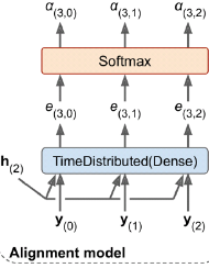
Figure 16-6. Neural machine translation using an Encoder–Decoder network with an attention model But where do these ![]() weights come from? It’s actually pretty simple: they are generated by a type of small neural network called an alignment model (or an attention layer), which is trained jointly with the rest of the Encoder–Decoder model. This alignment model is illustrated on the righthand side of Figure 16-6. It starts with a time-distributed Dense layer(Recall that a time-distributed Dense layer is equivalent to a regular Dense layer that you apply independently
weights come from? It’s actually pretty simple: they are generated by a type of small neural network called an alignment model (or an attention layer), which is trained jointly with the rest of the Encoder–Decoder model. This alignment model is illustrated on the righthand side of Figure 16-6. It starts with a time-distributed Dense layer(Recall that a time-distributed Dense layer is equivalent to a regular Dense layer that you apply independently
at each time step (only much faster).) with a single neuron, which receives as input all the encoder outputs, concatenated with the decoder’s previous hidden state (e.g., ![]() ). This layer outputs a score (or energy) for each encoder output (e.g.,
). This layer outputs a score (or energy) for each encoder output (e.g., ![]() ): this score measures how well each output
): this score measures how well each output![]() is aligned with the decoder’s previous hidden state
is aligned with the decoder’s previous hidden state
(###########################
why not use ![]() ? to be replaced by
? to be replaced by 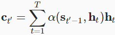
the RNN encoder transforms a variable-length sequence into a fixed-shape context variable, then the RNN decoder generates the output (target) sequence token by token based on the generated tokens and the context variable
( In general, the encoder transforms the hidden states at all the time steps into the context variable through a customized function q: ![]()
For example, when choosing ![]() such as in
such as in ![]() (We can use a function
(We can use a function ![]() to express the transformation of the RNN’s recurrent layer, e.g. LSTM or GRUhttps://blog.csdn.net/Linli522362242/article/details/114941730), the context variable is just the hidden state
to express the transformation of the RNN’s recurrent layer, e.g. LSTM or GRUhttps://blog.csdn.net/Linli522362242/article/details/114941730), the context variable is just the hidden state ![]() of the input sequence at the final time step(T).
of the input sequence at the final time step(T).
).
However, even though not all the input (source) tokens are useful for decoding a certain token( For example, the output of a layer for the word “Queen” in the sentence “They welcomed the Queen of the United Kingdom” will depend on all the words in the sentence, but it will probably pay more attention to the words “United” and “Kingdom” than to the words “They” or “welcomed.”), the same context variable that encodes the entire input sequence is still used at each decoding step.
In a separate but related challenge of handwriting generation for a given text sequence, Graves designed a differentiable attention model to align text characters with the much longer pen trace, where the alignment moves only in one direction [Graves, 2013]. Inspired by the idea of learning to align, Bahdanau et al. proposed a differentiable attention model without the severe unidirectional alignment limitation [Bahdanau et al., 2014]. When predicting a token, if not all the input tokens are relevant, the model aligns (or attends) only to parts of the input sequence that are relevant to the current prediction. This is achieved by treating the context variable as an output of attention pooling.
context variable c in (9.7.3) is replaced by ![]() at any decoding time step
at any decoding time step ![]() . Suppose that there are T tokens in the input sequence, the context variable at the decoding time step
. Suppose that there are T tokens in the input sequence, the context variable at the decoding time step ![]() is the output of attention pooling:
is the output of attention pooling:
where the decoder hidden state ![]() at time step
at time step ![]() −1 is the query, and the encoder hidden states
−1 is the query, and the encoder hidden states ![]() (are both the keys and values)
(are both the keys and values)
(e.g. In LSTM cells![]() OR GRU
OR GRU The hidden state of the encoder in time step t is the output of time step t)
and the attention weight α is computed as in the follow:
In general, when queries![]() and keys
and keys![]() are vectors of different lengths, we can use additive attention as the scoring function. Given a query
are vectors of different lengths, we can use additive attention as the scoring function. Given a query ![]() and a key
and a key ![]() , the additive attention scoring function
, the additive attention scoring function![]() (10.3.3)
(10.3.3)
where learnable parameters ![]() ,
, ![]() , and
, and ![]() . Equivalent to (10.3.3), the query and the key are concatenated and fed into an MLP with a single hidden layer whose number of hidden units is h, a hyperparameter. By using tanh as the activation function and disabling bias terms,
. Equivalent to (10.3.3), the query and the key are concatenated and fed into an MLP with a single hidden layer whose number of hidden units is h, a hyperparameter. By using tanh as the activation function and disabling bias terms,
Slightly different from the vanilla RNN encoder-decoder architecture in Fig. 9.7.2, the same architecture with Bahdanau attention is depicted in Fig. 10.4.1. Fig. 10.4.1 Layers in an RNN encoder-decoder model with Bahdanau attention.
 Fig. 9.7.2 Layers in an RNN encoder-decoder model.
implement the RNN decoder with Bahdanau attention. The state of the decoder is initialized with
- i) the encoder final-layer hidden states at all the time steps (as keys and values of the attention
 );
); - ii) the encoder all-layer hidden state at the final time step (to initialize the hidden state of the decoder : encoder RNN layer to decoder RNN layer); and
- iii) the encoder valid length (to exclude the padding tokens in attention pooling).
At each decoding time step, the decoder final-layer hidden state at the previous time step is used as the query of the attention. As a result, both the attention output and the input embedding(Targets) are concatenated as the input of the RNN decoder.
###########################). Finally, all the scores
![]() go through a softmax layer to get a final weight for each encoder output (e.g.,
go through a softmax layer to get a final weight for each encoder output (e.g., ![]() ). All the weights for a given decoder time step add up to 1 (since the softmax layer is not time-distributed). This particular attention mechanism is called Bahdanau attention (named after the paper’s first author). Since it concatenates the encoder output with the decoder’s previous hidden state, it is sometimes called concatenative attention (or additive attention).
). All the weights for a given decoder time step add up to 1 (since the softmax layer is not time-distributed). This particular attention mechanism is called Bahdanau attention (named after the paper’s first author). Since it concatenates the encoder output with the decoder’s previous hidden state, it is sometimes called concatenative attention (or additive attention).
If the input sentence is n words long, and assuming the output sentence is about as long(假设输出句子的长度大约为n个单词), then this model will need to compute about ![]() weights. Fortunately, this quadratic computational complexity is still tractable because even long sentences don’t have thousands of words.
weights. Fortunately, this quadratic computational complexity is still tractable because even long sentences don’t have thousands of words.
concatenative attention(additive attention) is much less used now
Another common attention mechanism was proposed shortly after, in a 2015 paper( Minh-Thang Luong et al., “Effective Approaches to Attention-Based Neural Machine Translation,” Proceedings of the 2015 Conference on Empirical Methods in Natural Language Processing (2015): 1412–1421. ) by Minh-Thang Luong et al. Because the goal of the attention mechanism is to measure the similarity between one of the encoder’s outputs(ORencoder final-layer hidden states at all the time steps) and the decoder’s(final-layer) previous hidden state,
- the authors proposed to simply compute the dot product (see Cp4 https://blog.csdn.net/Linli522362242/article/details/104005906) of these two vectors, as this is often a fairly good similarity measure, and modern hardware can compute it much faster. For this to be possible, both vectors must have the same dimensionality. This is called Luong attention (again, after the paper’s first author), or sometimes multiplicative attention. The dot product gives a score, and all the scores (at a given decoder time step) go through a softmax layer to give the final weights, just like in Bahdanau attention.
- Another simplification they proposed was to use the decoder’s hidden state at the current time step rather than at the previous time step (i.e.,
 ) rather than
  , e.g. ,
  and y_t ==> decoder's LSTM OR GRU==>), then to use the output of the attention mechanism (noted
  ) directly to compute the decoder’s predictions (rather than using it to compute the decoder’s current hidden state).
 - They also proposed a variant of the dot product mechanism where the encoder outputs first go through a linear transformation (i.e., a time-distributed Dense layer without a bias term) before the dot products are computed. This is called the “general” dot product approach. They compared both dot product approaches to the concatenative attention mechanism (adding a rescaling parameter vector v), and they observed that the dot product variants performed better than concatenative attention(concatenates the encoder output with the decoder’s previous hidden state). For this reason, concatenative attention is much less used now. The equations for these three attention mechanisms are summarized in Equation 16-1.
Equation 16-1. Attention mechanisms
Here is how you can add Luong attention to an Encoder–Decoder model using TensorFlow Addons:
attention_mechanism = tfa.seq2seq.attention_wrapper.LuongAttention(
    units, encoder_state, memory_sequence_length=encoder_sequence_length)
attention_decoder_cell = tfa.seq2seq.attention_wrapper.AttentionWrapper(
    decoder_cell, attention_mechanism, attention_layer_size=n_units)
We simply wrap the decoder cell in an AttentionWrapper, and we provide the desired attention mechanism (Luong attention in this example).
########################################################
Queries, Keys, and Values
Inspired by the nonvolitional非意志性的,非自愿 and volitional[və'lɪʃnəl] attention cues that explain the attentional deployment, in the following we will describe a framework for designing attention mechanisms by incorporating these two attention cues.
To begin with, consider the simpler case where only nonvolitional cues are available. To bias selection over sensory inputs, we can simply use a parameterized fully-connected layer or even non-parameterized max or average pooling.
Therefore, what sets attention mechanisms apart from those fully-connected layers or pooling layers is the inclusion of the volitional cues. In the context of attention mechanisms, we refer to volitional cues as queries. Given any query, attention mechanisms bias selection over sensory inputs (e.g., intermediate feature representations) via attention pooling. These sensory inputs are called values in the context of attention mechanisms. More generally, every value is paired with a key, which can be thought of the nonvolitional cue of that sensory input. As shown in Fig. 10.1.3, we can design attention pooling so that the given query (volitional cue) can interact with keys (nonvolitional cues), which guides bias selection over values (sensory inputs). Fig. 10.1.3 Attention mechanisms bias selection over values (sensory inputs) via attention pooling, which incorporates queries (volitional cues) and keys (nonvolitional cues).
Note that there are many alternatives for the design of attention mechanisms. For instance, we can design a non-differentiable attention model that can be trained using reinforcement learning methods [Mnih et al., 2014]. Given the dominance of the framework in Fig. 10.1.3, models under this framework will be the center of our attention in this chapter.
Attention Pooling: Nadaraya-Watson Kernel Regression
Now you know the major components of attention mechanisms under the framework in Fig. 10.1.3. To recapitulate, the interactions between queries (volitional cues) and keys (nonvolitional cues) result in attention pooling. The attention pooling selectively aggregates values (sensory inputs e.g., intermediate feature representations) to produce the output. In this section, we will describe attention pooling in greater detail to give you a high-level view of how attention mechanisms work in practice. Specifically, the Nadaraya-Watson kernel regression model proposed in 1964 is a simple yet complete example for demonstrating machine learning with attention mechanisms.
Average Pooling
We begin with perhaps the world’s “dumbest” estimator for this regression problem: using average pooling to average over all the training outputs: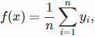 (10.2.2)
Nonparametric Attention Pooling
Obviously, average pooling omits the inputs ![]() . A better idea was proposed by Nadaraya [Nadaraya, 1964] and Waston [Watson, 1964] to weigh the outputs
. A better idea was proposed by Nadaraya [Nadaraya, 1964] and Waston [Watson, 1964] to weigh the outputs ![]() according to their input locations:
according to their input locations: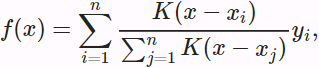 (10.2.3)
where K is a kernel. The estimator in (10.2.3) is called Nadaraya-Watson kernel regression. Here we will not dive into details of kernels. Recall the framework of attention mechanisms in Fig. 10.1.3. From the perspective of attention, we can rewrite (10.2.3) in a more generalized form of attention pooling: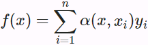 (10.2.4)
where ![]() is the query and
is the query and ![]() is the key-value pair. Comparing (10.2.4) and (10.2.2), the attention pooling here is a weighted average of values
is the key-value pair. Comparing (10.2.4) and (10.2.2), the attention pooling here is a weighted average of values ![]() . The attention weight
. The attention weight ![]() in (10.2.4) is assigned to the corresponding value
in (10.2.4) is assigned to the corresponding value ![]() based on the interaction between the query
based on the interaction between the query ![]() and the key
and the key ![]() modeled by
modeled by ![]() . For any query, its attention weights over all the key-value pairs are a valid probability distribution: they are non-negative and sum up to one.
. For any query, its attention weights over all the key-value pairs are a valid probability distribution: they are non-negative and sum up to one.
To gain intuitions of attention pooling, just consider a Gaussian kernel defined as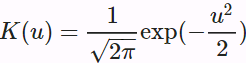 <==
<== https://blog.csdn.net/Linli522362242/article/details/105196037
Plugging the Gaussian kernel into (10.2.4) and (10.2.3) gives(10.2.6)<==Softmax function : https://blog.csdn.net/Linli522362242/article/details/104124771
In (10.2.6), a key ![]() that is closer to the given query
that is closer to the given query ![]() will get more attention via a larger attention weight assigned to the key’s corresponding value
will get more attention via a larger attention weight assigned to the key’s corresponding value ![]() .
.
Notably, Nadaraya-Watson kernel regression is a nonparametric model; thus (10.2.6) is an example of nonparametric attention pooling.
Parametric Attention Pooling
Nonparametric Nadaraya-Watson kernel regression enjoys the consistency benefit: given enough data this model converges to the optimal solution. Nonetheless, we can easily integrate learnable parameters into attention pooling.
As an example, slightly different from (10.2.6), in the following the distance between the query ![]() and the key
and the key ![]() is multiplied a learnable parameter
is multiplied a learnable parameter ![]() :
: (10.2.7)
we used a Gaussian kernel to model interactions between queries and keys. Treating the exponent of the Gaussian kernel in (10.2.6) as an attention scoring function (or scoring function for short), the results of this function were essentially fed into a softmax operation. As a result, we obtained a probability distribution (attention weights) over values that are paired with keys. In the end, the output of the attention pooling is simply a weighted sum of the values based on these attention weights.
########################################################
Visual Attention
Attention mechanisms are now used for a variety of purposes. One of their first applications beyond NMT(Neural machine translation) was in generating image captions using visual attention:(Kelvin Xu et al., “Show, Attend and Tell: Neural Image Caption Generation with Visual Attention,” Proceedings of the 32nd International Conference on Machine Learning (2015): 2048–2057.) a convolutional neural network first processes the image and outputs some feature maps, then a decoder RNN equipped with an attention mechanism generates the caption, one word at a time. At each decoder time step (each word), the decoder uses the attention model to focus on just the right part of the image. For example, in Figure 16-7, the model generated the caption “A woman is throwing a frisbee飞盘 in a park,” and you can see what part of the input image the decoder focused its attention on when it was about to output the word “frisbee”: clearly, most of its attention was focused on the frisbee. Figure 16-7. Visual attention: an input image (left) and the model’s focus before producing the word “frisbee” (right)(This is a part of figure 3 from the paper. It is reproduced with the kind authorization of the authors.)
#################################
Explainability
One extra benefit of attention mechanisms is that they make it easier to understand what led the model to produce its output. This is called explainability. It can be especially useful when the model makes a mistake: for example, if an image of a dog walking in the snow is labeled as “a wolf walking in the snow,” then you can go back and check what the model focused on when it output the word “wolf.” You may find that it was paying attention not only to the dog, but also to the snow, hinting at a possible explanation: perhaps the way the model learned to distinguish dogs from wolves is by checking whether or not there’s a lot of snow around. You can then fix this by training the model with more images of wolves without snow, and dogs with snow. This example comes from a great 2016 paper (Marco Tulio Ribeiro et al., “‘Why Should I Trust You?’: Explaining the Predictions of Any Classifier,” Proceedings of the 22nd ACM SIGKDD International Conference on Knowledge Discovery and Data Mining (2016): 1135–1144.) by Marco Tulio Ribeiro et al. that uses a different approach to explainability: learning an interpretable model locally around a classifier’s prediction.
In some applications, explainability is not just a tool to debug a model; it can be a legal requirement (think of a system deciding whether or not it should grant you a loan).
#################################
Attention mechanisms are so powerful that you can actually build state-of-the-art models using only attention mechanisms.
Attention Is All You Need: The Transformer Architecture
In a groundbreaking 2017 paper(Ashish Vaswani et al., “Attention Is All You Need,” Proceedings of the 31st International Conference on Neural Information Processing Systems (2017): 6000–6010.), a team of Google researchers suggested that “Attention Is All You Need.” They managed to create an architecture called the Transformer, which significantly improved the state of the art in NMT without using any recurrent or convolutional layers(Since the Transformer uses time-distributed Dense layers, you could argue that it uses 1D convolutional layers with a kernel size of 1.), just attention mechanisms (plus embedding layers, dense layers, normalization layers, and a few other bits and pieces). As an extra bonus, this architecture was also much faster to train and easier to parallelize, so they managed to train it at a fraction of the time and cost of the previous state-of-the-art models.
The Transformer architecture is represented in Figure 16-8. VS
VS Figure 16-8. The Transformer architecture (This is figure 1 from the paper, reproduced with the kind authorization of the authors.)
Let’s walk through this figure:
- • The lefthand part is the encoder. Just like earlier, it takes as input a batch of sentences represented as sequences of word IDs (the input shape is [batch size, max input sentence length]), and it encodes each word into a 512-dimensional representation (so the encoder’s output shape is [batch size, max input sentence length, 512]). Note that the top part of the encoder is stacked N times (in the paper, N = 6).
- • The righthand part is the decoder.
During training, it takes the target sentence as input (also represented as a sequence of word IDs), shifted one time step to the right (i.e., a start-of-sequence token is inserted at the beginning). It also receives the outputs of the encoder (i.e., the arrows coming from the left side). Note that the top part of the decoder is also stacked N times, and the encoder stack’s final outputs are fed to the decoder at each of these N levels. Just like earlier, the decoder outputs a probability for each possible next word, at each time step (its output shape is [batch size, max output sentence length, vocabulary length]).
- • During inference, the decoder cannot be fed targets, so we feed it the previously output words (starting with a start-of-sequence token). So the model needs to be called repeatedly, predicting one more word at every round (which is fed to the decoder at the next round, until the end-of-sequence token is output).
-
• Looking more closely, you can see that you are already familiar with most components: there are
2 embedding layers,
5 × N skip connections, each of them followed by a layer normalization layer,
2 × N “Feed Forward” modules that are composed of 2 dense layers each (the first one using the ReLU activation function, the second with no activation function), and
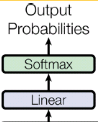
finally the output layer is a dense layer using the softmax activation function.
All of these layers are timedistributed, so each word is treated independently of all the others. But how can we translate a sentence by only looking at one word at a time? Well, that’s where the new components come in:
—The encoder’s Multi-Head Attention layer encodes each word’s relationship with every other word in the same sentence, paying more attention to the most relevant ones.
For example, the output of this layer for the word “Queen” in the sentence “They welcomed the Queen of the United Kingdom” will depend on all the words in the sentence, but it will probably pay more attention to the words “United” and “Kingdom” than to the words “They” or “welcomed.”
This attention mechanism is called self-attention (the sentence is paying attention to itself). We will discuss exactly how it works shortly. The decoder’s Masked Multi-Head Attention layer does the same thing, but each word is only allowed to attend to words located before it.
Finally, the decoder’s upper Multi-Head Attention layer is where the decoder pays attention to the words in the input sentence.
For example, the decoder will probably pay close attention to the word “Queen” in the input sentence when it is about to output this word’s translation.
—The positional embeddings are simply dense vectors (much like word embeddings) that represent the position of a word in the sentence. The positional embedding is added to the word embedding of the
  word in each sentence. This gives the model access to each word’s position, which is needed because the Multi-Head Attention layers do not consider the order or the position of the words; they only look at their relationships. Since all the other layers are time-distributed, they have no way of knowing the position of each word (either relative or absolute). Obviously, the relative and absolute word positions are important, so we need to give this information to the Transformer somehow, and positional embeddings are a good way to do this.
Let’s look a bit closer at both these novel components of the Transformer architecture, starting with the positional embeddings.
###########################
Attention Scoring Functions(10.2.6)<==Softmax function : https://blog.csdn.net/Linli522362242/article/details/104124771
we used a Gaussian kernel to model interactions between queries and keys. Treating the exponent of the Gaussian kernel in (10.2.6) as an attention scoring function (or scoring function for short), the results of this function were essentially fed into a softmax operation. As a result, we obtained a probability distribution (attention weights) over values that are paired with keys. In the end, the output of the attention pooling is simply a weighted sum of the values based on these attention weights.
At a high level, we can use the above algorithm to instantiate the framework of attention mechanisms in Fig. 10.1.3. Denoting an attention scoring function by ![]() , Fig. 10.3.1 illustrates how the output of attention pooling can be computed as a weighted sum of values. Since attention weights are a probability distribution, the weighted sum is essentially a weighted average.
, Fig. 10.3.1 illustrates how the output of attention pooling can be computed as a weighted sum of values. Since attention weights are a probability distribution, the weighted sum is essentially a weighted average. Fig. 10.3.1 Computing the output of attention pooling as a weighted average of values.
Mathematically, suppose that we have a query ![]() and m key-value pairs
and m key-value pairs ![]() , where any
, where any ![]() and any
and any ![]() . The attention pooling
. The attention pooling ![]() is instantiated as a weighted sum of the values:
is instantiated as a weighted sum of the values:![]()
where the attention weight (scalar) for the query ![]() and key
and key ![]() is computed by the softmax operation of an attention scoring function
is computed by the softmax operation of an attention scoring function ![]() that maps two vectors to a scalar:
that maps two vectors to a scalar:![]() As we can see, different choices of the attention scoring function
As we can see, different choices of the attention scoring function ![]() lead to different behaviors of attention pooling.
lead to different behaviors of attention pooling.
Masked Softmax Operation
As we just mentioned, a softmax operation is used to output a probability distribution as attention weights. In some cases, not all the values should be fed into attention pooling. For instance, for efficient minibatch processing in https://blog.csdn.net/Linli522362242/article/details/115518150, some text sequences are padded with special tokens that do not carry meaning. To get an attention pooling over only meaningful tokens as values, we can specify a valid sequence length (in number of tokens) to filter out those beyond this specified range when computing softmax.
Additive Attention
In general, when queries![]() and keys
and keys![]() are vectors of different lengths, we can use additive attention as the scoring function. Given a query
are vectors of different lengths, we can use additive attention as the scoring function. Given a query ![]() and a key
and a key ![]() , the additive attention scoring function
, the additive attention scoring function![]() (10.3.3)
(10.3.3)
where learnable parameters ![]() ,
, ![]() , and
, and ![]() . Equivalent to (10.3.3), the query and the key are concatenated and fed into an MLP with a single hidden layer whose number of hidden units is
. Equivalent to (10.3.3), the query and the key are concatenated and fed into an MLP with a single hidden layer whose number of hidden units is ![]() , a hyperparameter. By using tanh as the activation function and disabling bias terms,
, a hyperparameter. By using tanh as the activation function and disabling bias terms,
每个英文单词或者一个中国文字都有一个数值索引来表示,单词的索引是X(key), 中国文字的索引是target(实际Value,也是要预测的值),通过model来预测值(也就是我们平时要查询一个英文单字的中文含义):Each English word or a Chinese character has a numerical index to indicate that the index of the word is X (key), and the index of the Chinese character is target (the actual value, which is also the value to be predicted), and the value is predicted by the model. (That is, we usually need to check the Chinese meaning of an English word)
Scaled Dot-Product Attention
A more computationally efficient design for the scoring function can be simply dot product. However, the dot product operation requires that both the query and the key have the same vector length, say d. Assume that all the elements of the query and the key are independent random variables with zero mean and unit variance. The dot product of both vectors has zero mean and a variance of d. To ensure that the variance of the dot product still remains one regardless of vector length, the scaled dot-product attention scoring function![]()
divides the dot product by ![]() . In practice, we often think in minibatches for efficiency, such as computing attention for n queries and m key-value pairs, where queries and keys are of length d and values are of length v. The scaled dot-product attention of queries
. In practice, we often think in minibatches for efficiency, such as computing attention for n queries and m key-value pairs, where queries and keys are of length d and values are of length v. The scaled dot-product attention of queries ![]() , keys
, keys ![]() , and values
, and values ![]() is
is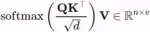
Multi-Head Attention
In practice, given the same set of queries, keys, and values we may want our model to combine knowledge from different behaviors of the same attention mechanism, such as capturing dependencies of various ranges (e.g., shorter-range vs. longer-range) within a sequence. Thus, it may be beneficial to allow our attention mechanism to jointly use different representation subspaces of queries, keys, and values.
To this end, instead of performing a single attention pooling, queries, keys, and values can be transformed with ![]() independently learned linear projections. Then these
independently learned linear projections. Then these ![]() projected queries, keys, and values are fed into attention pooling in parallel. In the end,
projected queries, keys, and values are fed into attention pooling in parallel. In the end, ![]() attention pooling outputs are concatenated and transformed with another learned linear projection to produce the final output. This design is called multi-head attention, where each of the
attention pooling outputs are concatenated and transformed with another learned linear projection to produce the final output. This design is called multi-head attention, where each of the ![]() attention pooling outputs is a head [Vaswani et al., 2017]. Using fully-connected layers to perform learnable linear transformations, Fig. 10.5.1 describes multi-head attention.
attention pooling outputs is a head [Vaswani et al., 2017]. Using fully-connected layers to perform learnable linear transformations, Fig. 10.5.1 describes multi-head attention. Fig. 10.5.1 Multi-head attention, where multiple heads are concatenated then linearly transformed.
Model
Before providing the implementation of multi-head attention, let us formalize this model mathematically. Given a query ![]() , a key
, a key ![]() , and a value
, and a value ![]() , each attention head
, each attention head ![]() is computed as
is computed as![]()
where learnable parameters ![]() and
and ![]() , and
, and ![]() is attention pooling, such as additive attention and scaled dot-product attention. The multi-head attention output is another linear transformation via learnable parameters
is attention pooling, such as additive attention and scaled dot-product attention. The multi-head attention output is another linear transformation via learnable parameters ![]() of the concatenation of
of the concatenation of ![]() heads:
heads: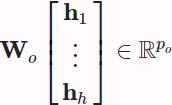 ......
Based on this design, each head may attend to different parts of the input. More sophisticated functions than the simple weighted average can be expressed.
In deep learning, we often use CNNs or RNNs to encode a sequence. Now with attention mechanisms. imagine that we feed a sequence of tokens into attention pooling so that the same set of tokens act as queries, keys, and values. Specifically, each query attends to all the key-value pairs and generates one attention output. Since the queries, keys, and values come from the same place, this performs self-attention [Lin et al., 2017b][Vaswani et al., 2017], which is also called intra-attention [Cheng et al., 2016][Parikh et al., 2016][Paulus et al., 2017]. In this section, we will discuss sequence encoding using self-attention, including using additional information for the sequence order.
Self-Attention
Given a sequence of input tokens ![]() where any
where any ![]() , its self-attention outputs a sequence of the same length
, its self-attention outputs a sequence of the same length ![]() , where
, where![]() 10.6.1 <==10.2.4
10.6.1 <==10.2.4
according to the definition of attention pooling ![]() in (10.2.4). Using multi-head attention to compute the self-attention of a tensor with shape (batch size, number of time steps or sequence length in tokens, d). The output tensor has the same shape.
in (10.2.4). Using multi-head attention to compute the self-attention of a tensor with shape (batch size, number of time steps or sequence length in tokens, d). The output tensor has the same shape.
Comparing CNNs, RNNs, and Self-Attention
Let us compare architectures for mapping a sequence of n tokens to another sequence of equal length, where each input or output token is represented by a d-dimensional vector. Specifically, we will consider CNNs, RNNs, and self-attention. We will compare their computational complexity, sequential operations, and maximum path lengths. Note that sequential operations prevent parallel computation, while a shorter path between any combination of sequence positions makes it easier to learn long-range dependencies within the sequence [Hochreiter et al., 2001]. Fig. 10.6.1 Comparing CNN (padding tokens are omitted), RNN, and self-attention architectures.
Consider a convolutional layer whose kernel size is k(1D kernel size=kx1). We will provide more details about sequence processing using CNNs in later chapters. For now, we only need to know that since the sequence length is n(size of 1D input feature maps=nx1), the numbers of input and output channels(OR the number of feature maps) are both d, the computational complexity of the convolutional layer is ![]() <==O(kx1 x nx1x dxd). As Fig. 10.6.1 shows, CNNs are hierarchical so there are
<==O(kx1 x nx1x dxd). As Fig. 10.6.1 shows, CNNs are hierarchical so there are ![]() sequential operations and the maximum path length is
sequential operations and the maximum path length is ![]() . For example,
. For example, ![]() and
and ![]() are within the receptive field of a two-layer CNN with kernel size 3
are within the receptive field of a two-layer CNN with kernel size 3 ![]() in Fig. 10.6.1.https://zhuanlan.zhihu.com/p/31575074
in Fig. 10.6.1.https://zhuanlan.zhihu.com/p/31575074
When updating the hidden state of RNNs, multiplication of the d×d weight matrix and the d-dimensional hidden state has a computational complexity of ![]() . Since the sequence length is n, the computational complexity of the recurrent layer is
. Since the sequence length is n, the computational complexity of the recurrent layer is ![]() . According to Fig. 10.6.1, there are
. According to Fig. 10.6.1, there are ![]() sequential operations that cannot be parallelized and the maximum path length is also
sequential operations that cannot be parallelized and the maximum path length is also ![]() .
.
In self-attention, the queries, keys, and values are all n×d matrices. Consider the scaled dot-product attention in (10.3.5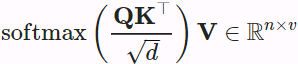 , where a n×d matrix is multiplied by a d×n matrix, then the output n×n matrix is multiplied by a n×d matrix. As a result, the self-attention has a
 ![]() <==O(n×
<==O(n×d x d×n x n×d xn <==![]() )computational complexity. As we can see in Fig. 10.6.1, each token is directly connected to any other token via self-attention. Therefore, computation can be parallel with
)computational complexity. As we can see in Fig. 10.6.1, each token is directly connected to any other token via self-attention. Therefore, computation can be parallel with ![]() sequential operations and the maximum path length is also
sequential operations and the maximum path length is also ![]() .
.
自注意力包括三个步骤:相似度计算、softmax和加权求和。相似度计算的时间复杂度是 ![]() ),因为可以看成(n,d)和(d,n)两个矩阵的相乘。softmax的时间复杂度是
),因为可以看成(n,d)和(d,n)两个矩阵的相乘。softmax的时间复杂度是![]() 。加权求和的时间复杂度是
。加权求和的时间复杂度是![]() ,同样可以看成(n,n)和(n,d)的矩阵相乘。
,同样可以看成(n,n)和(n,d)的矩阵相乘。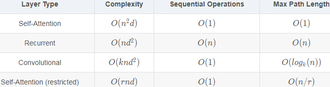
All in all, both CNNs and self-attention enjoy parallel computation![]() and self-attention has the shortest maximum path length
and self-attention has the shortest maximum path length![]() . However, the quadratic computational complexity
. However, the quadratic computational complexity![]() with respect to the sequence length makes self-attention prohibitively slow for very long sequences(n, 模型在序列长度过长时表现不如RNN,不过在可并行性和处理长依赖的能力上具有绝对的优势。我们的任务,就是想办法尽可能用词向量维度来弥补长度的劣势,只要d < n d < nd<n,那么模型的性能也是杠杠的。
with respect to the sequence length makes self-attention prohibitively slow for very long sequences(n, 模型在序列长度过长时表现不如RNN,不过在可并行性和处理长依赖的能力上具有绝对的优势。我们的任务,就是想办法尽可能用词向量维度来弥补长度的劣势,只要d < n d < nd<n,那么模型的性能也是杠杠的。
Positional Encoding
Unlike RNNs that recurrently process tokens of a sequence one by one, self-attention ditches sequential operations in favor of parallel computation. To use the sequence order information, we can inject absolute or relative positional information by adding positional encoding to the input representations. Positional encodings can be either learned or fixed. In the following, we describe a fixed positional encoding based on sine and cosine functions [Vaswani et al., 2017].
Suppose that the input representation X∈![]() contains the d-dimensional embeddings for n tokens of a sequence. The positional encoding outputs X+P using a positional embedding matrix P∈
contains the d-dimensional embeddings for n tokens of a sequence. The positional encoding outputs X+P using a positional embedding matrix P∈![]() of the same shape, whose element on the
of the same shape, whose element on the ![]() row and the
row and the ![]() or the
or the ![]() column is
column is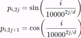 (10.6.2)
In the positional embedding matrix P, rows correspond to positions within a sequence and columns represent different positional encoding dimensions. In the example below, we can see that the 6th and the 7th columns(higher d) of the positional embedding matrix have a higher frequency than the 8th and the 9th columns(lower d). The offset![]() between the 6th and the 7th (same for the 8th and the 9th) columns is due to the alternation of sine and cosine functions(different component of the embedding).
between the 6th and the 7th (same for the 8th and the 9th) columns is due to the alternation of sine and cosine functions(different component of the embedding).
- At the same position in the sentence (sequence), different component of the embedding (different functions, eg sine or cosine function) get different PE values;
- the same component of the embedding (same function), but different positions in the sentence (sequence) , the PE value obtained maybe same. In other words, for the same PE value in the same component of the embedding (same function), the positions in the sentence (sequence) maybe different, so we need different function to distinguish this case.
To see how the monotonically[mɒnə'tɒnɪklɪ单调地 decreased frequency along the encoding dimension relates to absolute positional information, let us print out the binary representations of 0,1,…,7. As we can see, the lowest bit, the second-lowest bit, and the third-lowest bit alternate on every number, every two numbers, and every four numbers, respectively.
In binary representations, a higher bit has a lower frequency than a lower bit. Similarly, as demonstrated in the heat map below, the positional encoding decreases frequencies along the encoding dimension by using trigonometric functions. Since the outputs are float numbers, such continuous representations are more space-efficient than binary representations.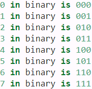 VS
VS
Relative Positional Information
Besides capturing absolute positional information, the above positional encoding also allows a model to easily learn to attend by relative positions. This is because for any fixed position offset ![]() , the positional encoding at position
, the positional encoding at position ![]() can be represented by a linear projection of that at position
can be represented by a linear projection of that at position ![]() .
.
This projection can be explained mathematically. Denoting ![]() , any pair of
, any pair of ![]() in (10.6.2 ) can be linearly projected to
in (10.6.2 ) can be linearly projected to ![]() for any fixed offset
for any fixed offset ![]() :
:
where the 2×2 projection matrix does not depend on any position index ![]() .
.
###########################
Positional embeddings
A positional embedding is a dense vector that encodes the position of a word within a sentence: the ![]() positional embedding is simply added to the word embedding of the
positional embedding is simply added to the word embedding of the ![]() word in the sentence. These positional embeddings can be learned by the model, but in the paper the authors preferred to use fixed positional embeddings, defined using the sine and cosine functions of different frequencies. The positional embedding matrix P is defined in Equation 16-2 and represented at the bottom of Figure 16-9 (transposed), where
word in the sentence. These positional embeddings can be learned by the model, but in the paper the authors preferred to use fixed positional embeddings, defined using the sine and cosine functions of different frequencies. The positional embedding matrix P is defined in Equation 16-2 and represented at the bottom of Figure 16-9 (transposed), where ![]() is the
is the ![]() component of the embedding for the word located at the
component of the embedding for the word located at the ![]() position in the sentence.
position in the sentence.
Equation 16-2. Sine/cosine positional embeddings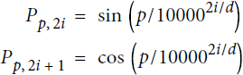
 Figure 16-9. Sine/cosine positional embedding matrix (transposed, top) with a focus on
two values of i (bottom)
- At the same position in the sentence (sequence), different component of the embedding (different functions, eg sine or cosine function) get different PE values;
- the same component of the embedding (same function), but different positions in the sentence (sequence) , the PE value obtained maybe same. In other words, for the same PE value in the same component of the embedding (same function), the positions in the sentence (sequence) maybe different, so we need different function to distinguish this case.
- In binary representations, a higher bit has a lower frequency than a lower bit. Similarly, as demonstrated in the heat map below, the positional encoding decreases frequencies(decreases width of the same color stripes) along the encoding dimension by using trigonometric functions. Since the outputs are float numbers, such continuous representations are more space-efficient than binary representations.
This solution gives the same performance as learned positional embeddings do, but it can extend to arbitrarily long sentences, which is why it’s favored. After the positional embeddings are added to the word embeddings, the rest of the model has access to the absolute position of each word in the sentence because there is a unique positional embedding for each position (e.g., the positional embedding for the word located at the 22nd position in a sentence is represented by the vertical dashed line at the bottom left of Figure 16-9, and you can see that it is unique to that position). Moreover, the choice of oscillating functions (sine and cosine) makes it possible for the model to learn relative positions as well. For example, words located 38 words apart (e.g., at positions p = 22 and p = 60) always have the same positional embedding values in the embedding dimensions i = 100 and i = 101, as you can see in Figure 16-9. This explains why we need both the sine and the cosine for each frequency: if we only used the sine (the blue wave at i = 100), the model would not be able to distinguish positions p = 25 and p = 35 (marked by a cross).
There is no PositionalEmbedding layer in TensorFlow, but it is easy to create one. For efficiency reasons, we precompute the positional embedding matrix in the constructor (so we need to know the maximum sentence length, max_steps, and the number of dimensions for each word representation, max_dims). Then the call() method crops this embedding matrix to the size of the inputs, and it adds it to the inputs. Since we added an extra first dimension of size 1 when creating the positional embedding matrix, the rules of broadcasting will ensure that the matrix gets added to every sentence in the inputs:
Embeddings+Positional EmbeddingsVVVVVVVVVVVVVVVVVVVVVVVVVV

If we assumed the embedding has a dimensionality of 4(Embedding size=4), the actual positional encodings would look like this:

Attention Input Parameters — Query, Key, and Value
The Attention layer takes its input in the form of three parameters, known as the Query, Key, and Value.
All three parameters are similar in structure, with each word in the sequence represented by a vector(length=Embedding size).
from tensorflow import keras
import numpy as np
import tensorflow as tf

class PositionalEncoding( keras.layers.Layer):
    def __init__(self, max_steps, max_dims, dtype=tf.float32, **kwargs):
        super().__init__(dtype=dtype, **kwargs)
        if max_dims % 2==1:
            max_dims += 1 # max_dims must be even
        #p: the pth position in the sequence
        #i: the ith component of the embedding(sin function,cos function)
        p, i = np.meshgrid( np.arange(max_steps), #horizontal and be copied row by row
                            np.arange(max_dims//2)#vertical and be copied column by column
                          )#shape: pxi
        #(batch size, number of time steps or sequence length, d dimentions)
        pos_emb = np.empty( (1, max_steps, max_dims) )
                          # np.sin().shape==(i,p)==>.T==>shape(p,i)
        pos_emb[0,:, ::2] = np.sin( p/10000**(2*i/max_dims) ).T
        pos_emb[0,:, 1::2]= np.cos( p/10000**(2*i/max_dims) ).T
        self.positional_embedding = tf.constant(pos_emb.astype(self.dtype))

    def call(self, inputs):
        # inputs=np.zeros( (1, max_steps, max_dims), np.float32)
        shape = tf.shape(inputs)
        return inputs + self.positional_embedding[:, :shape[-2], :shape[-1]] # broad casting
max_steps = 201
max_dims = 512
pos_emb = PositionalEncoding( max_steps, max_dims )
PE = pos_emb( np.zeros( (1, max_steps, max_dims), np.float32)
)[0].numpy()import matplotlib.pyplot as plt
i1, i2, crop_i = 100, 101, 150
p1, p2, p3 = 22, 60, 35
fig, (ax2, ax1) = plt.subplots( nrows=2, ncols=1, #sharex=True,
figsize=(10,5) )
im=ax2.imshow( PE.T[:crop_i], cmap="gray",
interpolation="bilinear", aspect="auto" )
ax2.hlines( i1,
0, max_steps-1, color="b" )##########################
cheat = 2 # need to raise the yellow line a bit,
# or else it hides the blue one
ax2.hlines( i2+cheat,
0, max_steps-1, color="y" )##########################
ax2.plot( [p1, p1],
[0, crop_i], "k--" )
ax2.plot( [p2, p2],
[0, crop_i], "k--", alpha=0.5 )
ax2.plot( [p1, p2], [i2+cheat, i2+cheat], "yo")
ax2.plot( [p1, p2], [i1, i1], "bo" )
ax2.axis( [0, max_steps - 1,
0, crop_i] )
ax2.set_ylabel( "$i$",rotation=0, fontsize=16 )
from mpl_toolkits.axes_grid1 import make_axes_locatable
divider = make_axes_locatable(ax2)
cax = divider.append_axes('right', size='6%', pad=0.1) # 200*0.06=12
cb = fig.colorbar(im, cax=cax, orientation="vertical")
cb.set_ticks([-1,0,1])
cb.update_ticks()
# p: the pth position in the sequence
# i: the ith component of the embedding
ax1.plot( PE[:, i1], "b-", label="$i = {}$".format(i1) )#########
ax1.plot( PE[:, i2], "y-", label="$i = {}$".format(i2) )#########
ax1.plot( [p1, p2], [ PE[p1, i1], PE[p2, i1] ], "bo" )
ax1.plot( [p1, p2], [ PE[p1, i2], PE[p2, i2] ], "yo" )
ax1.plot( p3, PE[p3, i1], "bx", label="$p = {}$".format(p3) )
ax1.plot( [p1, p1],
[-1, 1], "k--", label="$p = {}$".format(p1) )
ax1.plot( [p2, p2],
[-1, 1], "k--", label="$p = {}$".format(p2), alpha=0.5 )
ax1.legend( loc="center right", fontsize=14, framealpha=0.95 )
ax1.set_ylabel("$P_{(p,i)}$", rotation=0, fontsize=16 )
ax1.grid(True, alpha=0.3)
ax1.hlines( 0,
0,max_steps-1, color="k", linewidth=1, alpha=0.3 )
ax1.axis( [ 0, 215,# must >max_steps-1+12
-1, 1] )
ax1.set_xlabel( "Position in sequence", fontsize=16)
plt.show()
Then we can create the first layers of the Transformer: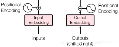
embed_size = 512
max_steps = 500
vocab_size = 10000

embeddings = keras.layers.Embedding(vocab_size, embed_size)
positional_encoding = PositionalEncoding( max_steps, max_dims=embed_size )

encoder_inputs = keras.layers.Input( shape=[None], # None: timesteps
                                     dtype=np.int32 )
encoder_embeddings = embeddings( encoder_inputs )
encoder_in = positional_encoding( encoder_embeddings )

decoder_inputs = keras.layers.Input( shape=[None], #None: OR sequences
                                     dtype=np.int32 )
decoder_embeddings = embeddings( decoder_inputs )
decoder_in = positional_encoding( decoder_embeddings )^^^^^^^^^^^^^^^^^^^^^^^^^Embeddings+Positional Embeddings^^^^^^^^^^^^^^^^^^^^^^^^^
Now let’s look deeper into the heart of the Transformer model: the Multi-Head Attention layer.
Multi-Head Attention
To understand how a Multi-Head Attention layer works, we must first understand the Scaled Dot-Product Attention layer, which it is based on. Let’s suppose the encoder analyzed the input sentence “They played chess,” and it managed to understand that the word “They” is the subject and the word “played” is the verb, so it encoded this information in the representations of these words. Now suppose the decoder has already translated the subject, and it thinks that it should translate the verb next. For this, it needs to fetch the verb from the input sentence. This is analog['ænəlɔg模拟 to a dictionary lookup: it’s as if the encoder created a dictionary {“subject”: “They”, “verb”: “played”, …} and the decoder wanted to look up the value that corresponds to the key “verb.” However, the model does not have discrete tokens to represent the keys (like “subject” or “verb”); it has vectorized representations of these concepts (which it learned during training), so the key it will use for the lookup (called the query) will not perfectly match any key in the dictionary. The solution is to
- compute a similarity measure between the query and each key in the dictionary, and then
- use the softmax function to convert these similarity scores to weights that add up to 1.
- If the key that represents the verb is by far the most similar to the query, then that key’s weight will be close to 1. Then the model can compute a weighted sum of the corresponding values, so if the weight of the “verb” key is close to 1, then the weighted sum will be very close to the representation of the word “played.”
In short, you can think of this whole process as a differentiable dictionary lookup. The similarity measure used by the Transformer is just the dot product, like in Luong attention. In fact, the equation is the same as for Luong attention, except for a scaling factor. The equation is shown in Equation 16-3, in a vectorized form.
Equation 16-3. Scaled Dot-Product Attention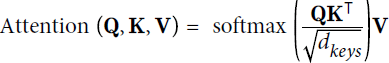
In this equation:
- • Q is a matrix containing one row per query. Its shape is
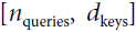 , where
  is the number of queries and
  is the number of dimensions of each query and each key.
 - • K is a matrix containing one row per key. Its shape is
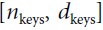 , where
  is the number of keys and values.
 - • V is a matrix containing one row per value. Its shape is
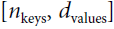 , where
  is the number of each value.
 - • The shape of
 is
is  : it contains one similarity score for each query/key pair. The output of the softmax function(to find the highest similarity score between each given query and ) has the same shape, but all rows sum up to 1(all re). The final output has a shape of
  : there is one row per query, where each row represents the query result (a weighted sum of the values).
 - • The scaling factor scales down the similarity scores to avoid saturating the softmax function, which would lead to tiny gradients.
- • It is possible to mask out some key/value pairs by adding a very large negative value to the corresponding similarity scores, just before computing the softmax. This is useful in the Masked Multi-Head Attention layer.
In the encoder, this equation is applied to every input sentence in the batch, with Q, K, and V all equal to the list of words in the input sentence(Embeddings+Positional Embeddings) (so each word in the sentence will be compared to every word in the same sentence, including itself). ![]() ==>Similarly, in the decoder’s masked attention layer, the equation will be applied to every target sentence in the batch, with Q, K, and V all equal to the list of words in the target sentence, but this time using a mask to prevent any word from comparing itself to words located after it (at inference time the decoder will only have access to the words it already output, not to future words, so during training we must mask out future output tokens). In the upper attention layer of the decoder, the keys K and values V are simply the list of word encodings produced by the encoder, and the queries Q are the list of word encodings produced by the decoder.
==>Similarly, in the decoder’s masked attention layer, the equation will be applied to every target sentence in the batch, with Q, K, and V all equal to the list of words in the target sentence, but this time using a mask to prevent any word from comparing itself to words located after it (at inference time the decoder will only have access to the words it already output, not to future words, so during training we must mask out future output tokens). In the upper attention layer of the decoder, the keys K and values V are simply the list of word encodings produced by the encoder, and the queries Q are the list of word encodings produced by the decoder.
The keras.layers.Attention layer implements Scaled Dot-Product Attention, efficiently applying Equation 16-3 to multiple sentences in a batch. Its inputs are just like Q, K, and V, except with an extra batch dimension (the first dimension).
###############################
In TensorFlow, if A and B are tensors with more than two dimensions—say, of shape [2, 3, 4, 5] and [2, 3, 5, 6] respectively—then tf.matmul(A, B) will treat these tensors as 2 × 3 arrays where each cell contains a matrix, and it will multiply the corresponding matrices: the matrix at the ![]() row and
row and ![]() column in A will be multiplied by the matrix at the
column in A will be multiplied by the matrix at the ![]() row and
row and ![]() column in B. Since the product of a 4 × 5 matrix with a 5 × 6 matrix is a 4 × 6 matrix, tf.matmul(A, B) will return an array of shape [2, 3, 4, 6].
column in B. Since the product of a 4 × 5 matrix with a 5 × 6 matrix is a 4 × 6 matrix, tf.matmul(A, B) will return an array of shape [2, 3, 4, 6].
###############################
If we ignore the skip connections, the layer normalization layers, the Feed Forward blocks, and the fact that this is Scaled Dot-Product Attention, not exactly Multi-Head Attention, then the rest of the Transformer model can be implemented like this:
Here is a (very) simplified Transformer (the actual architecture has skip connections, layer norm, dense nets, and most importantly it uses Multi-Head Attention instead of regular Attention):
Self-Attention and Decoder Self-Attention VVVVVVVVVVVVVVVVVVVVVVVVVVVVVVVVVVVVVVVV
Attention Input Parameters — Query, Key, and Value
The Attention layer takes its input in the form of three parameters, known as the Query, Key, and Value.
All three parameters are similar in structure, with each word in the sequence represented by a vector(length=Embedding size).
Encoder Self-Attention
The input sequence is fed to the Input Embedding and Position Encoding, which produces an encoded representation for each word in the input sequence that captures the meaning and position of each word. This is fed to all three parameters, Query, Key, and Value(All three parameters are similar in structure, with each word in the sequence represented by a vector.) in the Self-Attention in the first Encoder which then also produces an encoded representation for each word in the input sequence, that now incorporates the attention scores for each word as well. As this passes through all the Encoders in the stack, each Self-Attention module also adds its own attention scores into each word’s representation.
Along with that, the output of the final Encoder in the stack is passed to the Value and Key parameters in the Encoder-Decoder Attention.
Decoder Self-Attention
Coming to the Decoder stack, the target sequence is fed to the Output Embedding and Position Encoding, which produces an encoded representation for each word in the target sequence that captures the meaning and position of each word. This is fed to all three parameters, Query, Key, and Value(All three parameters are similar in structure, with each word in the sequence represented by a vector.) in the Self-Attention in the first Decoder which then also produces an encoded representation for each word in the input sequence, that now incorporates the attention scores for each word as well.
After passing through the Layer Norm, this is fed to the Query parameter in the Encoder-Decoder Attention in the first Decoder.
Encoder-Decoder Attention
The Encoder-Decoder Attention is therefore getting a representation of both the target sequence (from the Decoder Self-Attention) and a representation of the input sequence (from the Encoder stack). It, therefore, produces a representation with the attention scores for each target sequence word that captures the influence of the attention scores from the input sequence as well.
As this passes through all the Decoders in the stack, each Self-Attention and each Encoder-Decoder Attention also add their own attention scores into each word’s representation.

In the encoder, this equation is applied to every input sentence in the batch, with Q, K, and V all equal to the list of words in the input sentence(Embeddings+Positional Embeddings) (so each word in the sentence will be compared to every word in the same sentence, including itself).
######################create a Query vector, a Key vector, and a Value vector.
Linear Layers
There are three separate Linear layers for the Query, Key, and Value. Each Linear layer has its own weights. The input(=output of Input embeding+Positional Encoding) is passed through these Linear layers to produce the Q, K, and V matrices.
If you want to change Embedding Dimentions, you must use a Conv1D. This step must be before entering the self-attention layer.
https://www.tensorflow.org/api_docs/python/tf/keras/layers/Attention
https://blog.csdn.net/Linli522362242/article/details/108414534
# CNN layer.
cnn_layer = tf.keras.layers.Conv1D(
    filters=64, #### use filters to change embedding dimensions###############
    kernel_size=1,#####weight matrix
    # Use 'same' padding so outputs have the same shape as inputs. # Here is Tq OR Tv
    padding='same',
    use_bias=False
)
# Query encoding of shape [batch_size, Tq, filters].
query_seq_encoding = cnn_layer(query_embeddings)
# Value encoding of shape [batch_size, Tv, filters].
value_seq_encoding = cnn_layer(value_embeddings)
# Key encoding of shape [batch_size, Tv, filters].
key_seq_encoding = cnn_layer(key_embeddings)
X1 : 1x1 with dimensions=4(channels, feature maps) and X2 : 1x1 with dimensions=4(channels)
All weights: 1x1(kernel_size) x input feature maps(![]() =4) x output feature maps(
=4) x output feature maps(![]() =3)
=3)
 (conv_layer: https://blog.csdn.net/Linli522362242/article/details/108414534)
OR counstruct WQ weight matrix, WK matrix, WV matrix by ourself
Notice that these new vectors are smaller in dimension than the embedding vector. Their dimensionality is 64, while the embedding and encoder input/output vectors have dimensionality of 512. They don’t HAVE to be smaller, this is an architecture choice to make the computation of multiheaded attention (mostly) constant. <==
<==
Multiplying x1 by the WQ weight matrix produces q1, the "query" vector associated with that word. We end up creating a "query", a "key", and a "value" projection of each word in the input sentence.
This softmax score determines how much each word will be expressed at this position. Clearly the word at this position will have the highest softmax score, but sometimes it’s useful to attend to another word that is relevant to the current word.
The fifth step is to multiply each value vector by the softmax score (in preparation to sum them up). The intuition here is to keep intact the values of the word(s) we want to focus on, and drown-out irrelevant words (by multiplying them by tiny numbers like 0.001, for example).
The sixth step is to sum up the weighted value vectors. This produces the output of the self-attention layer at this position (for the first word). <==
<==![]() <==
<==
######################http://jalammar.github.io/illustrated-transformer/
^^^^^^^^^^^^^^^^^^^^^^^ Self-Attention and Decoder Self-Attention ^^^^^^^^^^^^^^^^^^^^^^^
# encoder_in = positional_encoding(encoder_embeddings)
Z = encoder_in
# Z are query, value and key
# query: [batch_size, Tq, dim]
# value: [batch_size, Tv, dim]
# if key: [batch_size, Tv, dim]
for N in range(6):
    # The use_scale=True argument creates an additional parameter that
    # lets the layer learn how to properly downscale the similarity scores.
                      # input:( [query_seq_encoding, value_seq_encoding])
    Z = keras.layers.Attention( use_scale=True )([Z,Z])  # OR ([Z,Z,Z])
# # Query-value attention of shape [batch_size, Tq, dim].

encoder_outputs=Z
# decoder_in = positional_encoding( decoder_embeddings )
Z = decoder_in
for N in range(6):
    # The causal=True argument ensures that each output token
    # only attends to previous output tokens, not future ones.
    Z = keras.layers.Attention( use_scale=True, causal=True )( [Z,Z] )
    Z = keras.layers.Attention( use_scale=True )([Z, encoder_outputs])
outputs = keras.layers.TimeDistributed(
                    keras.layers.Dense( vocab_size, activation="softmax")
          )(Z)
The use_scale=True argument creates an additional parameter that lets the layer learn how to properly downscale the similarity scores. This is a bit different from the Transformer model, which always downscales the similarity scores by the same factor ( ![]() ). The causal=True argument when creating the second attention layer
). The causal=True argument when creating the second attention layer
ensures that each output token only attends to previous output tokens, not future ones(prevent any word from comparing itself to words located after it (at inference time the decoder will only have access to the words it already output, not to future words, so during training we must mask out future output tokens).).
Now it’s time to look at the final piece of the puzzle: what is a Multi-Head Attention layer? Its architecture is shown in Figure 16-10. Attention
Multiple Attention Heads
In the Transformer, the Attention module repeats its computations multiple times in parallel. Each of these is called an Attention Head. The Attention module splits its Query, Key, and Value parameters N-ways and passes each split independently through a separate Head. All of these similar Attention calculations are then combined together to produce a final Attention score. This is called Multi-head attention and gives the Transformer greater power to encode multiple relationships and nuances for each word. VS
VS Figure 16-10. Multi-Head Attention layer architecture(This is the right part of figure 2 from the paper, reproduced with the kind authorization of the authors.)
As you can see, it is just a bunch of Scaled Dot-Product Attention layers, each preceded by a linear transformation of the values, keys, and queries (i.e., a timedistributed Dense layer with no activation function). All the outputs are simply concatenated, and they go through a final linear transformation (again, timedistributed). But why? What is the intuition behind this architecture? Well, consider the word “played” we discussed earlier (in the sentence “They played chess”). The encoder was smart enough to encode the fact that it is a verb. But the word representation also includes its position in the text, thanks to the positional encodings, and it probably includes many other features that are useful for its translation, such as the fact that it is in the past tense过去式. In short, the word representation encodes many different characteristics of the word. If we just used a single Scaled Dot-Product Attention layer, we would only be able to query all of these characteristics in one shot. This is why the Multi-Head Attention layer applies multiple different linear transformations of the values, keys, and queries: this allows the model to apply many different projections of the word representation into different subspaces, each focusing on a subset of the word’s characteristics. Perhaps one of the linear layers will project the word representation into a subspace where all that remains is the information that the word is a verb, another linear layer will extract just the fact that it is past tense, and so on. Then the Scaled Dot-Product Attention layers implement the lookup phase, and finally we concatenate all the results and project them back to the original space.
At the time of this writing, there is no Transformer class or MultiHeadAttention class available for TensorFlow 2. However, you can check out TensorFlow’s great tutorial for building a Transformer model for language understanding. Moreover, the TF Hub team is currently porting several Transformer-based modules to TensorFlow 2, and they should be available soon. In the meantime, I hope I have demonstrated that it is not that hard to implement a Transformer yourself, and it is certainly a great exercise!
Attention Hyperparameters
There are three hyperparameters that determine the data dimensions:
- Embedding Size — width of the embedding vector (we use a width of 6 in our example). This dimension is carried forward throughout the Transformer model(contains N x encoder and N x decoder) and hence is sometimes referred to by other names like ‘model size’ etc.
- Query Size (equal to Key and Value size)— the size of the weights used by 3 Linear layers to produce the Query, Key, and Value matrices respectively (we use a Query size of 3 in our example)
- Number of Attention heads (we use 2 heads in our example)
In addition, we also have the Batch size, giving us one dimension for the number of samples.
Linear Layers
There are three separate Linear layers for the Query, Key, and Value. Each Linear layer has its own weights. The input(=output of Input embeding+Positional Encoding) is passed through these Linear layers to produce the Q, K, and V matrices.
Splitting data across Attention heads
Now the data gets split across the multiple Attention heads so that each can process it independently.
However, the important thing to understand is that this is a logical split only. The Query, Key, and Value are not physically split into separate matrices, one for each Attention head. A single data matrix is used for the Query, Key, and Value, respectively, with logically separate sections of the matrix for each Attention head. Similarly, there are not separate Linear layers, one for each Attention head. All the Attention heads share the same Linear layer but simply operate on their ‘own’ logical section of the data matrix.
Linear layer weights are logically partitioned per head
This logical split is done by partitioning the input data as well as the Linear layer weights uniformly across the Attention heads. We can achieve this by choosing the Query Size as below:
Query Size = Embedding Size / Number of heads For example
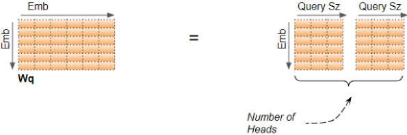
In our example, that is why the Query Size = Embedding Size / Number of heads = 6/2 = 3. Even though the layer weight (and input data) is a single matrix we can think of it as ‘stacking together’ the separate layer weights for each head.
The computations for all Heads can be therefore be achieved via a single matrix operation rather than requiring N separate operations. This makes the computations more efficient and keeps the model simple because fewer Linear layers are required, while still achieving the power of the independent Attention heads.
Reshaping the Q, K, and V matrices
The Q, K, and V matrices output by the Linear layers are reshaped to include an explicit Head dimension(Embedding Size==>(Number of heads, Query Size)). Now each ‘slice’ corresponds to a matrix per head.
This matrix is reshaped again by swapping the Head and Sequence dimensions. Although the Batch dimension is not drawn, the dimensions of Q are now (Batch, Head, Sequence, Query size). (Batch, Sequence, Head, Query size)==>(Batch, Head, Sequence, Query size)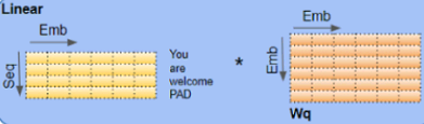 ==>
==>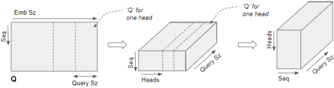
In the picture below, we can see the complete process of splitting our example Q matrix, after coming out of the Linear layer.
The final stage is for visualization only — although the Q matrix is a single matrix, we can think of it as a logically separate Q matrix per head.
Compute the Attention Score for each head
We now have the 3 matrices, Q, K, and V, split across the heads. These are used to compute the Attention Score.
We will show the computations for a single head using just the last two dimensions (Sequence and Query size) and skip the first two dimensions (Batch and Head). Essentially, we can imagine that the computations we’re looking at are getting ‘repeated’ for each head and for each sample in the batch (although, obviously, they are happening as a single matrix operation, and not as a loop).and ![]() is the Embedding Size
is the Embedding Size
- The first step is to do a matrix multiplication between Q and K.
- A Mask value is now added to the result. In the Encoder Self-attention, the mask is used to mask out the Padding values so that they don’t participate in the Attention Score (Note: since input sequences could be of different lengths they are extended with padding tokens like in most NLP applications so that fixed-length vectors can be input to the Transformer.).
 Different masks are applied in the Decoder Self-attention and in the Decoder Encoder-Attention which we’ll come to a little later in the flow.
 - The result is now scaled by dividing by the square root of the Query size, and then a Softmax is applied to it.
Embedding Size==>Embedding Size / Number of heads==>Query Size - Another matrix multiplication is performed between the output of the Softmax and the V matrix.
 ==>
==> ==>
==> ==>
==>
The complete Attention Score calculation in the Encoder Self-attention is as below:
 <==
<==
Merge each Head’s Attention Scores together
We now have separate Attention Scores for each head, which need to be combined together into a single score. This Merge operation is essentially the reverse of the Split operation.
It is done by simply reshaping the result matrix to eliminate the Head dimension. The steps are:
- Reshape the Attention Score matrix by swapping the Head and Sequence dimensions. In other words, the matrix shape goes from (Batch, Head, Sequence, Query size) to (Batch, Sequence, Head, Query size).
- Collapse the Head dimension by reshaping to (Batch, Sequence, Head * Query size). This effectively concatenates the Attention Score vectors for each head into a single merged Attention Score.
Since Embedding size =Head * Query size, the merged Score is (Batch, Sequence, Embedding size). In the picture below, we can see the complete process of merging for the example Score matrix.
End-to-end Multi-head Attention
Putting it all together, this is the end-to-end flow of the Multi-head Attention.

Multi-head split captures richer interpretations
An Embedding vector(the result of input Embeddings+Positional Embeddings) captures the meaning of a word. In the case of Multi-head Attention, as we have seen, the Embedding vectors for the input (and target) sequence gets logically split across multiple heads. What is the significance of this? 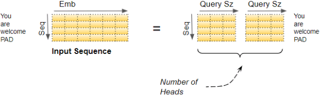 This means that separate sections of the Embedding can learn different aspects of the meanings of each word, as it relates to other words in the sequence. This allows the Transformer to capture richer interpretations of the sequence.
This may not be a realistic example, but it might help to build intuition. For instance, one section might capture the ‘gender-ness’ (male, female, neuter) of a noun while another might capture the ‘cardinality’ (singular vs plural)“基数”(单数或复数) of a noun. This might be important during translation because, in many languages, the verb that needs to be used depends on these factors.
K = keras.backend

class MultiHeadAttention( keras.layers.Layer ):
    def __init__(self, n_heads, causal=False, use_scale=False, **kwargs):
        self.n_heads = n_heads
        self.causal = causal
        self.use_scale = use_scale
        super().__init__(**kwargs)

    def build(self, batch_input_shape):
        self.dims = batch_input_shape[0][-1]
                   # Query Size = Embedding Size / Number of heads
        self.q_dims, self.v_dims, self.k_dims = [self.dims // self.n_heads]*3 # could be hyperparameters instead
        # (batch size, number of time steps or sequence length in tokens, d dimentions)
        # d dimensions in the Conv1D is n_filters and sum all filters up for each cell(seq)
        # Linear layer
        self.q_linear = keras.layers.Conv1D( self.n_heads * self.q_dims, # filters=Embedding Size
                                             kernel_size=1, # default strides=1, padding="valid"
                                             use_bias=False )
        self.v_linear = keras.layers.Conv1D( self.n_heads * self.v_dims,
                                             kernel_size=1,
                                             use_bias=False )
        self.k_linear = keras.layers.Conv1D( self.n_heads * self.k_dims,
                                             kernel_size=1,
                                             use_bias=False )
        # class BaseDenseAttention(Layer):
        #      def call(self,inputs, mask=None, training=None, return_attention_scores=False):
        #           ... ...
        # https://github.com/tensorflow/tensorflow/blob/v2.4.1/tensorflow/python/keras/layers/dense_attention.py#L221-L355
        # class Attention(BaseDenseAttention):
        #      def _calculate_scores(self, query, key):
        #           """Calculates attention scores as a query-key dot product.
        #           scores = math_ops.matmul(query, key, transpose_b=True)
        #           if self.scale is not None:
        #                scores *= self.scale
        #           return scores
        # Q * K.T/sqrt(q_dims or Embedding Size)
        self.attention = keras.layers.Attention( causal=self.causal, use_scale=self.use_scale )
        # Linear layer
        self.out_linear = keras.layers.Conv1D( self.dims, kernel_size=1, use_bias=False )
        super().build(batch_input_shape)

    def _multi_head_linear(self, inputs, linear):
        # split
        # inputs shape : 3D( batch size, number of time steps or sequence length, d dimentions )
        shape = K.concatenate([ K.shape(inputs)[:-1], # except dims(or Embedding Size)
                                [self.n_heads, -1] # =[self.n_heads, self.q_dims OR self.v_dims
                              ])# axis=-1          #                 OR self.k_dims]
        projected = K.reshape( linear(inputs), # flatten
                               shape )
        # ==>4D( Batch_size, n_Sequence, n_heads, q_dims OR v_dims OR k_dims )
        # swap the Head and Sequence dimensions
        perm = K.permute_dimensions(projected, pattern=[0,2,1,3])
        # ==>4D( Batch_size, n_heads, n_Sequence, q_dims OR v_dims OR k_dims )
        return K.reshape( perm, [shape[0] * self.n_heads, shape[1], -1] )
        # since tf.keras only support 3D calculation
        # ==>3D( Batch_size * n_heads, n_Sequence, q_dims OR v_dims OR k_dims
    def call( self, inputs ):
        q = inputs[0]
        v = inputs[1]
        k = inputs[2] if len(inputs) > 2 else v
        shape = K.shape(q)
        q_proj = self._multi_head_linear( q, self.q_linear )
        v_proj = self._multi_head_linear( v, self.v_linear )
        k_proj = self._multi_head_linear( k, self.k_linear )
        # shape ==>3D( Batch_size * n_heads, n_Sequence, q_dims OR v_dims OR k_dims

        multi_attended = self.attention([q_proj, v_proj, k_proj]) # ==>  Attention Score
        # shape ==>3D( Batch_size * n_heads, n_Sequence, q_dims OR v_dims OR k_dims

        # Merge each Head’s Attention Scores together
        shape_attended = K.shape( multi_attended )
        reshape_attended = K.reshape( multi_attended,
                                      # Batch_size, n_heads,    n_Sequence, q_dims or Query size
                                      [ shape[0], self.n_heads, shape_attended[1], shape_attended[2]
                                    ])
        # Merge
        # swap the Head and Sequence dimensions
        perm = K.permute_dimensions( reshape_attended,
                                     pattern=[0,2,1,3] ) #==>(Batch, n_Sequence, n_heads, q_dims)
        concat = K.reshape(perm, [shape[0], shape_attended[1], -1])
        # Collapse the Head dimension by reshaping to (Batch, Sequence, Head * Query size)
        # ==>(Batch_size, n_Sequence, d dimentions OR Embedding Size)

        # Linear layer
        return self.out_linear(concat)
Q = np.random.rand(2, 50, 512)
V = np.random.rand(2, 80, 512)
multi_attn = MultiHeadAttention(8) #n_heads=8
multi_attn( [Q,V] ).shape 
Decoder Self-Attention and Masking
The Decoder Self-Attention works just like the Encoder Self-Attention, except that it operates on each word of the target sequence. <==
<==
Similarly, the Masking masks out the Padding words in the target sequence( The decoder’s Masked Multi-Head Attention layer does the same thing, but each word is only allowed to attend to words located before it.).masking serves to prevent the decoder from ‘peeking’ ahead at the rest of the target sentence when predicting the next word.
The Decoder processes words in the source sequence and uses them to predict the words in the destination sequence. During training, this is done via Teacher Forcing, where the complete target sequence is fed as Decoder inputs. Therefore, while predicting a word at a certain position, the Decoder has available to it the target words preceding that word as well as the target words following that word. This allows the Decoder to ‘cheat’ by using target words from future ‘time steps’.
at inference time, the output from the previous time step).
OR using a mask to prevent any word from comparing itself to words located after it (at inference time the decoder will only have access to the words it already output, not to future words, so during training we must mask out future output tokens). the Decoder masks out input words that appear later in the sequence.
For instance, when predicting ‘Word 3’, the Decoder should refer only to the first 3 input words from the target but not the fourth word ‘Ketan’.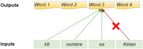
When calculating the Attention Score (refer to the picture earlier showing the calculations) masking is applied to the numerator just before the Softmax. The masked out elements (white squares) are set to negative infinity, so that Softmax turns those values to zero.
Encoder-Decoder Attention and Masking
The Encoder-Decoder Attention takes its input from two sources. Therefore, unlike the
- Encoder Self-Attention, which computes the interaction(or encodes the relationship) between each input word with other input words, and
- Decoder Self-Attention which computes the interaction between each target word with other target words,
- the Encoder-Decoder Attention computes the interaction between each target word with each input word.
 <==
<==
and the keys K and values V are simply the list of word encodings produced by the encoder, and the queries Q are the list of word encodings produced by the decoder.
Therefore each cell in the resulting Attention Score corresponds to the interaction between one Q (ie. target sequence word) with all other K (ie. input sequence) words and all V (ie. input sequence) words.
Similarly, the Masking masks out the later words in the target output
The Transformer architecture is represented in Figure 16-8.VSFigure 16-8. The Transformer architecture (This is figure 1 from the paper, reproduced with the kind authorization of the authors.)
Generate Output
- The last Decoder in the stack passes its output to the Output component which converts it into the final output sentence.
- The Linear layer projects the Decoder vector into Word Scores, with a score value for each unique word in the target vocabulary, at each position in the sentence. For instance, if our final output sentence has 7 words and the target Spanish vocabulary has 10000 unique words, we generate 10000 score values for each of those 7 words. The score values indicate the likelihood of occurrence for each word in the vocabulary in that position of the sentence.
- The Softmax layer then turns those scores into probabilities (which add up to 1.0).
- In each position, we find the index for the word with the highest probability, and
- then map that index to the corresponding word in the vocabulary. Those words then form the output sequence of the Transformer.

Training and Loss Function
During training, we use a loss function such as cross-entropy loss to compare the generated output probability distribution to the target sequence. The probability distribution gives the probability of each word occurring in that position. Let’s assume our target vocabulary contains just four words. Our goal is to produce a probability distribution that matches our expected target sequence “De nada END”.
This means that the probability distribution(in the target sequence) for the first word-position should have a probability of 1 for “De” with probabilities for all other words in the vocabulary being 0. Similarly, “nada” and “END” should have a probability of 1 for the second and third word-positions respectively.
As usual, the loss is used to compute gradients to train the Transformer via backpropagation.https://towardsdatascience.com/transformers-explained-visually-part-2-how-it-works-step-by-step-b49fa4a64f34
Recent Innovations in Language Models
The year 2018 has been called the “ImageNet moment for NLP”: progress was astounding使人震惊的, with larger and larger LSTM and Transformer-based architectures trained on immense巨大的 datasets. I highly recommend you check out the following papers, all published in 2018:
- The ELMo paper(Matthew Peters et al., “Deep Contextualized Word Representations,” Proceedings of the 2018 Conference of the North American Chapter of the Association for Computational Linguistics: Human Language Technologies 1 (2018): 2227–2237.) by Matthew Peters introduced Embeddings from Language Models (ELMo): these are contextualized word embeddings learned from the internal states of a deep bidirectional language model. For example, the word “queen” will not have the same embedding in “Queen of the United Kingdom” and in “queen bee.”
- The ULMFiT paper(Jeremy Howard and Sebastian Ruder, “Universal Language Model Fine-Tuning for Text Classification,” Proceedings of the 56th Annual Meeting of the Association for Computational Linguistics 1 (2018): 328–339.) by Jeremy Howard and Sebastian Ruder demonstrated the effectiveness of unsupervised pretraining for NLP tasks: the authors trained an LSTM language model using self-supervised learning (i.e., generating the labels automatically from the data) on a huge text corpus, then they fine-tuned it on various tasks. Their model outperformed the state of the art on six text classification tasks by a large margin大幅度 (reducing the error rate by 18–24% in most cases). Moreover, they showed that by fine-tuning the pretrained model on just 100 labeled examples, they could achieve the same performance as a model trained from scratch on 10,000 examples.
- The GPT paper(Alec Radford et al., “Improving Language Understanding by Generative Pre-Training” (2018).) by Alec Radford and other OpenAI researchers also demonstrated the effectiveness of unsupervised pretraining, but this time using a Transformer-like architecture. The authors pretrained a large but fairly simple architecture composed of a stack of 12 Transformer modules (using only Masked Multi-Head Attention layers) on a large dataset, once again trained using selfsupervised learning. Then they fine-tuned it on various language tasks, using only minor adaptations for each task仅对每个任务进行了少量修改. The tasks were quite diverse: they included text classification, entailment包含 (whether sentence A entails sentence B),(For example, the sentence “Jane had a lot of fun at her friend’s birthday party” entails “Jane enjoyed the party,” but it is contradicted与…发生矛盾 by “Everyone hated the party” and it is unrelated to “The Earth is flat.”) similarity (e.g., “Nice weather today” is very similar to “It is sunny”), and question answering (given a few paragraphs of text giving some context, the model must answer some multiple-choice questions). Just a few months later, in February 2019, Alec Radford, Jeffrey Wu, and other OpenAI researchers published the GPT-2 paper,(Alec Radford et al., “Language Models Are Unsupervised Multitask Learners” (2019).) which proposed a very similar architecture, but larger still (with over 1.5 billion parameters!) and they showed that it could achieve good performance on many tasks without any fine-tuning. This is called zero-shot learning (ZSL). A smaller version of the GPT-2 model (with “just” 117 million parameters) is available at https://github.com/openai/gpt-2, along with its pretrained weights.
- The BERT paper(Jacob Devlin et al., “BERT: Pre-training of Deep Bidirectional Transformers for Language Understanding,” Proceedings of the 2018 Conference of the North American Chapter of the Association for Computational Linguistics: Human Language Technologies 1 (2019).) by Jacob Devlin and other Google researchers also demonstrates the effectiveness of self-supervised pretraining on a large corpus, using a similar architecture to GPT but non-masked Multi-Head Attention layers (like in the Transformer’s encoder). This means that the model is naturally bidirectional; hence the B in BERT (Bidirectional Encoder Representations from Transformers). Most importantly, the authors proposed two pretraining tasks that explain most of the model’s strength:
Masked language model (MLM)
Each word in a sentence has a 15% probability of being masked, and the model is trained to predict the masked words. For example, if the original sentence is “She had fun at the birthday party,” then the model may be given the sentence “She <mask> fun at the <mask> party” and it must predict the words “had” and “birthday” (the other outputs will be ignored). To be more precise, each selected word has an 80% chance of being masked, a 10% chance of being replaced by a random word (to reduce the discrepancy差异 between pretraining and fine-tuning, since the model will not see <mask> tokens during fine-tuning), and a 10% chance of being left alone (to bias the model toward the correct answer).
Next sentence prediction (NSP)
The model is trained to predict whether two sentences are consecutive or not. For example, it should predict that “The dog sleeps” and “It snores loudly” are consecutive sentences, while “The dog sleeps” and “The Earth orbits在…轨道上运行,绕 the Sun” are not consecutive. This is a challenging task, and it significantly improves the performance of the model when it is fine-tuned on tasks such as question answering or entailment.
As you can see, the main innovations in 2018 and 2019 have been better subword tokenization, shifting from LSTMs to Transformers, and pretraining universal language models using self-supervised learning, then fine-tuning them with very few architectural changes (or none at all). Things are moving fast; no one can say what architectures will prevail next year. Today, it’s clearly Transformers, but tomorrow it might be CNNs (e.g., check out the 2018 paper(Maha Elbayad et al., “Pervasive Attention: 2D Convolutional Neural Networks for Sequence-to-Sequence Prediction,” arXiv preprint arXiv:1808.03867 (2018).) by Maha Elbayad et al., where the researchers use masked 2D convolutional layers for sequence-to-sequence tasks). Or it might even be RNNs, if they make a surprise comeback (e.g., check out the 2018 paper(Shuai Li et al., “Independently Recurrent Neural Network (IndRNN): Building a Longer and Deeper RNN,” Proceedings of the IEEE Conference on Computer Vision and Pattern Recognition (2018): 5457–5466.) by Shuai Li et al. that shows that by making neurons independent of each other in a given RNN layer, it is possible to train much deeper RNNs capable of learning much longer sequences).
In the next chapter we will discuss how to learn deep representations in an unsupervised way using autoencoders, and we will use generative adversarial networks
(GANs) to produce images and more!
Exercises
https://blog.csdn.net/Linli522362242/article/details/116065910


 237
237


 被折叠的 条评论
为什么被折叠?
被折叠的 条评论
为什么被折叠?
 到【灌水乐园】发言


