mpf10_yfinan_Explained variance_R2_ols_cointegration_Gradient Boost_lbfgs_热力图sns ticklabel_SVM_confu

LIQING LIN

已于 2022-09-14 19:06:00 修改

阅读量1.5k

点赞数 2

分类专栏： pythonForFinance pythonMachineLearningInAction 文章标签： big data python 大数据

于 2022-09-14 19:05:33 首次发布

本文链接：https://blog.csdn.net/Linli522362242/article/details/126672904

版权

pythonMachineLearningInAction 同时被 2 个专栏收录

101 篇文章 1 订阅

订阅专栏

pythonForFinance

75 篇文章 3 订阅

订阅专栏

Machine learning is being rapidly adopted for a range of applications in the financial services industry. The adoption of machine learning in financial services has been driven by both supply factors, such as technological advances in data storage, algorithms, and computing infrastructure, and by demand factors, such as profitability needs, competition with other firms, and supervisory and regulatory requirements. Machine learning in finance includes algorithmic trading, portfolio management, insurance underwriting保险承保, and fraud detection, just to name a few subject areas.

There are several types of machine learning algorithms, but the two main ones that you will commonly come across in machine learning literature are supervised and unsupervised machine learning. Our discussion in this chapter focuses on supervised learning. Supervised machine learning involves supplying both the input and output data to help the machine predict new input data. Supervised machine learning can be regression-based or classification-based. Regression-based machine learning algorithms predict continuous values, while classification-based machine learning algorithms predict a class or label.

In this chapter, we will be introduced to machine learning, study its concepts and applications in finance, and look at some practical examples for applying machine learning to assist in trading decisions. We will cover the following topics:

Explore the uses of machine learning in finance
Supervised and unsupervised machine learning
Classification-based and regression-based machine learning
Using scikit-learn for implementing machine learning algorithms
Applying single-asset regression-based machine learning in predicting prices
Understanding risk metrics风险指标 in measuring regression models
Applying multi-asset regression-based machine learning in predicting returns
Applying classification-based machine learning in predicting trends
Understanding risk metrics in measuring classification models

Introduction to machine learning

Before machine learning algorithms became mature, many software application decisions were rule-based, consisting of a bunch of if and else statements to generate the appropriate response in exchange to some input data. A commonly cited引用 example is a spam filter function in email inboxeshttps://blog.csdn.net/Linli522362242/article/details/93034532, https://blog.csdn.net/Linli522362242/article/details/120259487. A mailbox may contain blacklisted words黑名单的词 defined by a mail server administrator or owner. Incoming emails have their contents scanned against blacklisted words, and should the blacklist condition hold true, the mail is marked as spammed and sent to the Junk folder. As the nature of unwanted emails continues to evolve to avoid detection, spam filter mechanisms must also continuously update themselves to keep up with doing a better job. However, with machine learning, spam filters can automatically learn from past email data and, given an incoming email, calculate the possibility of classifying whether the new email is spam or not.

The algorithms behind facial recognition and image detection largely work in the same way. Digital images stored in bits and bytes are collected, analyzed, and classified according to expected responses provided by the owner. This process is known as training, using a supervised learning approach. The trained data may subsequently be used for predicting the next set of input data as some output response with a certain level of confidence. On the other hand, when the training data does not contain the expected response, the machine learning algorithm is expected to learn from the training data, and this process is called unsupervised learning.

Uses of machine learning in finance

Machine learning is increasingly finding its uses in many areas of finance, such as data security, customer service, forecasting, and financial services. A number of use cases leverage big data and artificial intelligence (AI) as well; they are not exclusive to machine learning. In this section, we will examine some of the ways in which machine learning is transforming the financial sector.

Algorithmic trading

Machine learning algorithms study the statistical properties of the prices of highly correlated assets, measure their predictive power on historical data during backtesting, and forecast prices to within certain accuracy(Prediction involves generating best estimates of in-sample data. Forecasting involves generating best estimates of out-of-sample data.). Machine learning trading algorithms may involve the analysis of

the order book,
market depth and volume,
news releases新闻发布, e
arnings calls财报会议(财报电话会议),
or financial statements财务报表,
where the analysis translates into price movement possibilities and is taken into account for generating trading signals.

Portfolio management

The concept of robo advisors机器人顾问 has been gaining popularity in recent years to act as automated hedge fund managers. They aid with portfolio construction, optimization, allocation, and rebalancing, and even suggest to clients the instruments to invest in based on their risk tolerance and preferred choice of investment vehicle. These advisories serve as a platform for interacting with a digital financial planner, providing financial advice and portfolio management.

Supervisory and regulatory functions

Financial institutions and regulators are adopting the use of AI and machine learning to analyze, identify, and flag suspicious/səˈspɪʃəs/感觉可疑的 transactions that warrant further investigation. Supervisors such as the Securities and Exchange Commission (SEC) take a data-driven approach and employ AI, machine learning, and natural language processing to identify behavior that warrants enforcement授权执行. Worldwide, central authorities中央当局 are developing machine learning capabilities in regulatory/ˈreɡjələtɔːri /监管的 functions.

Insurance and loan underwriting保险和贷款承保

Insurance companies actively use AI and machine learning to augment some insurance sector区域,部分 functions, improve pricing and marketing of insurance products, and to reduce claims索赔 processing times and operational costs. In loan underwriting承保, many data points of a single consumer, such as age, income, and credit score, are compared against a database of candidates in building credit risk profiles, determining credit scores, and calculating the possibility of loan defaults. Such data relies on transaction and payment history from financial institutions. However, lenders are increasingly turning to social media activities, mobile phone usage, and messaging activities to capture a more holistic/hoʊˈlɪstɪk/全面的 view of creditworthiness /ˈkredɪtwɜːrðinəs/有资格接受信用贷款,好信誉 speed up lending decisions, limit incremental risk, and improve the rating accuracy of loans.

News sentiment analysis新闻情绪分析

Natural language processing, a subset of machine learning, may be used to analyze alternative data, financial statements, news announcements, and even Twitter feeds, in creating investment sentiment indicators used by hedge funds, high-frequency trading firms, social trading, and investment platforms for analyzing markets in real time. Politicians' speeches, or important new releases, such as those made by central banks, are also being analyzed in real time, where each and every word is being scrutinized/ˈskruːtənaɪzd/详细检查的 and calculated to predict which asset prices could move and by how much. Machine learning will not only understand the movement of stock prices and trades, but also understand social media feeds, news trends, and other data sourceshttps://blog.csdn.net/Linli522362242/article/details/121172551.cp8_Sentiment_urlretrieve_pyprind_tarfile_bag词袋_walk目录_regex_verbose_N-gram_Hash_colab_verbose_文本向量化_LIQING LIN的博客-CSDN博客

Machine learning beyond finance

Machine learning is increasingly being employed in areas of facial recognition, voice recognition, biometrics, trade settlement贸易结算, chatbots, sales recommendations, content creation, and more. As machine learning algorithms improve and their rate of adoption picks up, the list of use cases becomes even longer.

Let's begin our journey in machine learning by understanding some of the terminology you will come across in the machine learning literature.

Supervised and unsupervised learning

There are many types of machine learning algorithms, but the two main ones that you will commonly come across are supervised and unsupervised machine learning.

Supervised learning

Supervised learning predicts a certain output from given inputs. These pairings of input to output data are known as training data. The quality of the prediction entirely depends on the training data; incorrect training data reduces the effectiveness of the machine learning model. An example is a dataset of transactions with labels identifying which ones are fraudulent/ˈfrɔːdʒələnt/欺诈的 , and which are not. A model can then be built to predict whether a new transaction will be fraudulent.

Some common algorithms in supervised learning are logistic regression, the support vector machine, and random forests.

Unsupervised learning

Unsupervised learning builds a model based on given input data that does not contain labels, but instead is asked to detect patterns in the data. This may involve identifying clusters of observations with similar underlying characteristics. Unsupervised learning aims to make accurate predictions to new, never-before-seen data.

For example, an unsupervised learning model may price illiquid非流动 securities by looking for a cluster of securities with similar characteristics. Common unsupervised learning algorithms include k-means clustering, principal component analysis, and autoencoders.

Classification and regression in supervised machine learning

There are two major types of supervised machine algorithms, mainly classification and regression.

Classification machine learning models attempt to predict and classify responses from a list of predefined possibilities. These predefined possibilities may be binary classification (such as a Yes or No response to a question: Is this email spam?) or multiclass classification.

Regression machine learning models attempt to predict continuous output values. For example, predicting housing prices or the temperature expects a continuous range of output values. Common forms of regressions are ordinary least squares (OLS) regression, LASSO regression, ridge regression, and elastic net regularization.

Overfitting and underfitting models

Poor performance in machine learning models can be caused by overfitting or underfitting.

https://blog.csdn.net/Linli522362242/article/details/96480059

An overfitted machine learning model is one that is trained too well with the training data such that it leads to negative performance on new data. This occurs when the training data is fitted to every minor variation, including noise and random fluctuations. Unsupervised learning algorithms are highly susceptible/səˈseptəb(ə)l/易受影响的 to overfitting, since the model learns from every piece of data, both good and bad.

An underfitted machine learning model gives poor accuracy of prediction. It may be caused by too little training data being available to build an accurate model, or that the data is not suitable for extracting its underlying trends数据不适合提取其潜在趋势. Underfitting models are easy to detect since they give consistently poor performance. To improve such models, provide more training data or use another machine learning algorithm.

Feature engineering

A feature is an attribute of the data that defines its characteristic. By using domain knowledge of the data, features can be created to help machine learning algorithms increase their predictive performance. This can be as simple as grouping or bucketing related parts of the existing data to form defining features. Even removing unwanted features is also feature engineering即使删除不需要的特征也是特征工程.

As an example, suppose we have the following time series price data that looks like this:

Grouping the time series into buckets by the hour of the day and taking the last price action in each bucket, we end up with a feature like this:

The process of feature engineering involves these four steps:

1. Brainstorming features to include in the training model
2. Creating those features
3. Checking how the features work with the model
4. Repeating from step 1 until the features work perfectly

There are absolutely no hard and fast rules when it comes to what constitutes creating features. Feature engineering is considered more of an art than a science.

Scikit-learn for machine learning

Scikit-learn is a Python library designed for scientific computing and contains a number of state-of-the-art machine learning algorithms for classification, regression, clustering, dimensionality reduction, model selection, and preprocessing. Its name is derived from the SciPy Toolkit, which is an extension of the SciPy module. Comprehensive documentation on scikit-learn can be found at https://scikit-learn.org/stable/.

SciPy is a collection of Python modules for scientific computing, containing a number of core packages, such as NumPy, Matplotlib, IPython, and others.

In this chapter, we will be using scikit-learn's machine learning algorithms to predict securities movements. Scikit-learn require a working installation of NumPy and SciPy. Install scikit-learn with the pip package manager by using the following command:

pip install scikit-learn

conda install scikit-learn

Predicting prices with a single-asset regression model使用单一资产回归模型预测价格

Pairs trading is a common statistical arbitrage trading strategy employed by traders using a pair of co-integrated协同整合 and highly positively correlated assets, though negatively correlated pairs can also be considered.

In this section, we will use machine learning to train regression-based models using the historical prices of a pair of securities that might be used in pairs trading. Given the current price of one security for a particular day, we predict the other security's price on a daily basis. The following examples uses the historical daily prices of Goldman Sachs (GS) and J.P. Morgan (JPM) traded on the New York Stock Exchange (NYSE). We will be predicting prices of JPM's stock price for the year 2018.

cointegration and correlation

to predict the prices of JPM using GS, with the assumption that the pair is cointegrated and highly correlated.

https://blog.csdn.net/Linli522362242/article/details/121721868

平稳性是很好用，但在现实中，绝大多数的股票都是非平稳的，那么我们是否还能够利用平稳性质进行获利呢？答案是肯定的，这时协整关系（cointegration）就出场了！如果两组序列是非平稳的，但它们的线性组合可以得到一个平稳序列，那么我们就说这两组时间序列数据具有协整的性质，我们同样可以把统计性质用到这个组合的序列上来。但是需要指出的一点，协整关系并不是相关关系（correlation)。

gs_jpm=df['Adj Close'].loc['2018-01-01':'2019-01-01']
gs_jpm

gs_jpm.plot()
plt.show()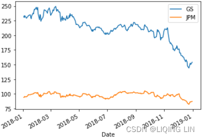

两组序列是非平稳的

cm = np.corrcoef( gs_jpm.values.T )
cm

But, their daily prices are existing a correlation

from statsmodels.tsa.stattools import coint

coin_t_statistic, pvalue, _ = coint( gs_jpm['GS'], gs_jpm['JPM'] )
pvalue

(the time series is not stationary) 显然，这两组数据都是非平稳的，因为均值随着时间的变化而变化。但这两组数据的daily change是具有协整关系（cointegration）的，因为他们的daily change 序列是平稳的：

gs_jpm.pct_change().plot()

plt.axhline( ( gs_jpm['JPM'].pct_change()
               #gs_jpm['GS'].pct_change()
             ).mean(),
             color="b", linestyle="--"
           )
plt.axhline( ( #gs_jpm['JPM'].pct_change()#-\
               gs_jpm['GS'].pct_change()
             ).mean(),
             color="k", linestyle="--"
           )

# plt.axhline( ( gs_jpm['JPM'].pct_change()-\
#                gs_jpm['GS'].pct_change()
#              ).mean(),
#              color="k", linestyle="-"
#            )
plt.show()

# pct_change() : prices-prices.shift(1)/prices.shift(1)
plt.plot( gs_jpm['JPM'].pct_change()-\
          gs_jpm['GS'].pct_change()
        )
plt.axhline( ( gs_jpm['JPM'].pct_change()-\
               gs_jpm['GS'].pct_change()
             ).mean(), 
             color="red", linestyle="--")
plt.xlabel("Time")
plt.ylabel("Price")
plt.legend(["JPM-GS", "Mean"])
plt.show()

上图中，可以看出蓝线一直围绕均值波动。而均值不随时间变化（其实方差也不随时间变化）他们的daily change 差序列也是平稳的

coin_t_statistic, pvalue, _ = coint( gs_jpm['GS'].pct_change().dropna(), 
                                     gs_jpm['JPM'].pct_change().dropna()
                                   )
pvalue

import numpy as np

cm = np.corrcoef(  gs_jpm['GS'].pct_change().dropna(),
                   gs_jpm['JPM'].pct_change().dropna()
                )
cm

their daily change is highly correlated(so we can predict the prices of JPM using GS)

Linear regression by OLS

Let's begin our investigation of regression-based machine learning with a simple linear regression model. A straight line is in the following form:
$\large \hat{y} = c + ax$ OR $\large \hat{y}(w,x )= w_0 + w_1x_1 + ... + w_px_p = \sum_{i=0}^{n} w_i x_i = w^Tx$ OR

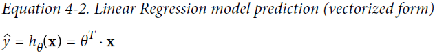
This attempts to fit the data by OLS:

$\large a = w = \theta$ is the coefficients(or the weight coefficients of the explanatory variable $\large x$ ) (coef_)
$\large c = w_0$ is the value of the y-intercept (intercept_) when $\large x_0 = 1$
x is a matrix containing all the features(excluding labels) of all instances in the dataset. There is one row per instance and the $\large i^{th}$ row containing n features
$\large \hat{y}$ is the predicted value from the straight line
Our goal is to learn the weights of the linear equation to describe the relationship between the explanatory variable $\large x$ and the target variable $\large y$ , which can then be used to predict the responses $\large \hat{y}$ of new explanatory variables that were not part of the training dataset.

one feature
two features

The coefficients and intercept are determined by minimizing the cost function:
$\large minimize \sum_{i=0}^{m-1} (y_i - \hat{y}_i )^2$ =m: the number of instances

minimize the residual sum of squares between the observed targets $\large y$ in the dataset, and the targets predicted $\large Xw$ (or $\large \hat{y}$ ) by the linear approximation.

==>minimizes: MSE(Mean Square Error) cost function for a Linear Regression model
minimizes:
==> minimizes RMSE(Root Mean Square Error)
minimizes: 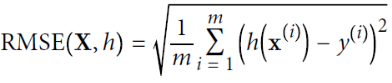==> need to find the value of θ or $\large w$ that minimizes the RMSE

note: the RMSE is more sensitive to outliers than the MAE( the sum of absolutes MAE(Mean Absolute Error, It is sometimes called the Manhattan norm) since the higher the norm index $\large k$ (the more it focuses on large values and neglects small ones). But when outliers are exponentially rare (like in a bell-shaped curve), the RMSE performs very well and is generally preferred.

y is the dataset of observed actual values(labels) used in performing a straight-line fit. In other words, we are performing a least sum of squared errors in finding the coefficients $\large a$ and $\large c$ , from which we can predict the current period.

Before developing a model, let's download and prepare the required datasets.

Preparing the independent and target variables

Let's obtain the datasets of GS and JPM prices with the following code:

import yfinance as yf

df = yf.download( 'JPM GS')
df

Goldman Sachs (GS) and J.P. Morgan (JPM)

Let's prepare our independent variables with the following code:

import pandas as pd

df_x = pd.DataFrame({ 'GS': df['Adj Close']['GS'] }).dropna()
df_x

The adjusted closing prices of GS are extracted to a new DataFrame object, df_x. Next, obtain our target variables with the following code:

jpm_prices = df['Adj Close']['JPM']
jpm_prices

The adjusted closing prices of JPM are extracted to the jpm_prices variable as a pandas Series object. Having prepared our datasets for use in modeling, let's proceed to develop the linear regression model.

Writing the linear regression model

(使用1个特征值('GS')的连续多个之前日期的adjusted closing prices作为样本训练当前日期的model，使用该模型对当前的jpm closing price进行预测。每个日期都有一个model对该日期进行预测jpm closing price)

We will create a class for using a linear regression model to fit and predict values. This class also serves as a base class for implementing other models in this chapter. The following steps illustrates this process.

1. Declare a class named LinearRegressionModel as follows:
In the constructor of our new class, we declare a pandas DataFrame called df_result to store the actual and predicted values for plotting on a chart later on.

The get_model() method returns an instance of the LinearRegression class in the sklearn.linear_model module for fitting and predicting the data.
The set fit_intercept parameter is set to True as the data is not centered (around 0 on the x- and y-axes, that is).
fit_intercept bool, default=True
Whether to calculate the intercept for this model. If set to False, no intercept will be used in calculations (i.e. data is expected to be centered).
if set to True, we will append a feature column which is filled with 1s.
normalize bool, default=False
This parameter is ignored when fit_intercept is set to False. If True, the regressors X will be normalized before regression by subtracting the mean and dividing by the l2-norm. If you wish to standardize, please use StandardScaler before calling fit on an estimator with normalize=False.

More information about the LinearRegression of scikit-learn can be found at https://scikit-learn.org/stable/modules/generated/sklearn.linear_model.LinearRegression.html

The get_prices_since() method slices a subset of the supplied dataset with the iloc command, from the given date index date_since and up to a number of earlier periods defined by the lookback value.

from sklearn.linear_model import LinearRegression
import numpy as np

class LinearRegressionModel( object ):
    def __init__(self):
        self.df_result = pd.DataFrame( columns=['Actual', 'Predicted'] )
        
    def get_model( self ):
        return LinearRegression( fit_intercept=False )
    
    def get_prices_since( self, df, date_since, lookback ):
        index = df.index.get_loc( date_since )
        return df.iloc[ index-lookback:index ]
    
    def learn( self, df, ys, start_date, end_date, lookback_period=20 ):
        model = self.get_model()
        
        df.sort_index( inplace=True )
        for date in df[start_date:end_date].index:
            
            # Fit the model
            x = self.get_prices_since( df, date, lookback_period )
            y = self.get_prices_since( ys, date, lookback_period )
            model.fit( x.values, y.ravel() )
            
            # Predict the current period
            x_current = df.loc[date].values # e.g. [232.54751587]
            
            [y_pred] = model.predict([x_current]) 
            #    [y_pred]=[93.2564989817077]
            # ==> y_pred = 93.2564989817077
            
            # Store predictions
            new_index = pd.to_datetime( date, format='%Y-%m-%d' )
            y_actual = ys.loc[date]
            
            self.df_result.loc[new_index] = [y_actual, y_pred]

2. The learn() method serves as the entry point for running the model. It accepts the df_x and ys parameters as our independent and target variables, start_date and end_date as strings corresponding to the index of the dataset for the period we will be predicting, and the lookback_period parameter as the number of historical data points used for fitting the model in the current period.

The for loop simulates a backtest on a daily basis. The call to get_prices_since() fetches a subset of the dataset for fitting the model on the x- and y-axes with the fit() command. The ravel() command transforms the given pandas Series object into a flattened list of target values for fitting the model.

The x_current variable represents independent variable values for the specified date, fed into the predict() method. The predicted output is a list object, from which we extract the first value. Both the actual and predicted values are saved to the df_result DataFrame, indexed by the current date as a pandas object.
3. Let's instantiate this class and run our machine learning model by issuing the following commands:
```
linear_reg_model = LinearRegressionModel()
linear_reg_model.learn( df_x, jpm_prices, 
                        start_date='2018-01-01', end_date='2019-01-01',
                        lookback_period=20
                      )

linear_reg_model.df_result
```
In the learn() command, we provided our prepared datasets, df_x and jpm_prices , and specified the prediction for the year of 2018. For this example, we assumed there are 20 trading days in a month. Using a lookback_period value of 20 , we are using a past month's prices to fit our model for prediction daily.
4. Let's retrieve the resulting df_result DataFrame from the model and plot both the actual and predicted values:
```
%matplotlib inline
import matplotlib.pyplot as plt

linear_reg_model.df_result.plot( title='JPM prediction by OLS',
                                 style=['b-', 'g--'],
                                 figsize=(12,8),
                               )
plt.show()
```
In the style parameter, we specified that actual values are to be drawn as a solid line, and predicted values drawn as dotted lines. This gives us the following graph:

The chart shows our predicted results trailing closely behind the actual values up to a certain extent. How well does our model actually perform? In the next section, we will discuss several common risk metrics for measuring regression-based models.

Risk metrics for measuring prediction performance

The sklearn.metrics module implements several regression metrics for measuring prediction performance. We will discuss the mean absolute error, the mean squared error, the explained variance score, and the $R^2$ score in subsequent sections.

Mean Absolute Error as a risk metric

The mean absolute error (MAE) is a risk metric that measures the average absolute prediction error and can be written as follows:
OR $\large MAE(y, \hat{y}) = \frac{1}{m}\sum_{i=0}^{m-1}\left | y_i - \hat{y}_i \right |$
Here, y and $\large \hat{y}$ are the actual and predicted lists of values, respectively, with the same length, m. and $\large \hat{y}_i$ are the predicted and $\large y_i$ actual values, respectively, at the index i. Taking the absolute values of errors means that our output results in a positive decimal value. Low values of MAE are highly desired. A perfect score of 0 implies that our prediction powers are exactly aligned with actual values, since there are no differences between the two.

Obtain the MAE value of our predictions using the mean_abolute_error function of the sklearn.metrics module with the following code:

from sklearn.metrics import mean_absolute_error

actual = linear_reg_model.df_result['Actual']
predicted = linear_reg_model.df_result['Predicted']

mae = mean_absolute_error( actual, predicted )
print('Mean Absolute Error:', mae)

The MAE of our linear regression model is 2.213.

Mean Squared Error as a risk metric

Like the MAE, the mean squared error (MSE) is a risk metric that measures the average of the squares of the prediction errors and can be written as follows:

$MSE(y, \hat{y}) = \frac{1}{m} \sum_{i=0}^{m-1} (y_i - \hat{y}_i)^2$ OR

Squaring the errors $(y_i - \hat{y}_i)^2$ means that values of MSE are always positive, and low values of MSE are highly desired. A perfect MSE score of 0 implies that our prediction powers are exactly aligned with actual values, and that the squares of such differences are negligible. While the application of both the MSE and MAE helps determine the strength of our model's predictive powers, MSE triumphs/ˈtraɪʌmfs/ over击败,得胜,成功 MAE by penalizing errors that are farther away from the mean(MSE通过惩罚远离均值的错误来战胜MAE). Squaring the errors places a heavier bias on the risk metrics(对误差进行平方会使风险指标产生更大的偏差).

Obtain the MSE value of our predictions using the mean_squared_error function of the sklearn. metrics module with the following code:

from sklearn.metrics import mean_squared_error

mse = mean_squared_error( actual, predicted )
print( 'Mean Squared Error:',mse )

The MSE of our linear regression model is 9.854 .

Explained variance score as a risk metric

The explained variance score explains the dispersion of errors of a given dataset解释给定数据集的误差分布, and the formula is written as follows:

Here, $Var( y - \hat{y} )$ and $Var(y)$ is the variance of prediction errors and actual values respectively. Scores close to 1.0 are highly desired, indicating better squares of standard deviations of errors.

Obtain the explained variance score of our predictions using the explained_variance_score function of the sklearn.metrics module with the following code:

from sklearn.metrics import explained_variance_score

eva = explained_variance_score( actual, predicted )
print( "Explained Variance Score:", eva )

The explained variance score of our linear regression model is 0.533.

R^2 $R^2$ as a risk metric

The $R^2$ score is also known as the coefficient of determination确定系数, and it measures how well future samples are likely to be predicted by the model. It is written as follows:
OR OR
Here, SSE is the sum of squared errors(OR the sum of squared of residuals)
and SST is the total sum of squares:In other words, SST is simply the variance of the response.

Here, $\large \bar{y}$ is the mean of actual values and can be written as follows:

Let's quickly show that is indeed just a rescaled version of the MSE:

$\large R^2 = 1 - \frac{SSE}{SST} = 1- \frac{ \frac{1}{n} \sum_{i=0}^{n-1}( y^{(i)} - \hat{y}^{(i)} )^2 }{ \frac{1}{n} \sum_{i=0}^{n-1}( y^{(i)} - u_y )^2 } = 1 - \frac{MSE}{Var(y)}$

$R^2$ scores ranges from negative values to 1.0.

A perfect $R^2$ score of 1 implies that there is no error in the regression analysis(the model fits the data perfectly with a corresponding MSE = 0(since Var(y)>0)),
the closer the value to 1, the better the fit
while a score of 0 indicates that the model always predicts the mean of target values.
the closer the value to 0, the worse the fit
A $\large R^2 < 0$ score indicates that the prediction performs below average.
Negative values mean that the model fits worse than the baseline model. Models with negative values usually indicate issues in the training data or process and cannot be used.

Obtain the $R^2$ score of our predictions using the r2_score function of the sklearn.metrics module with the following code:

from sklearn.metrics import r2_score

r2 = r2_score( actual, predicted )
print( 'r^2 score:', r2 )

The $R^2$ of our linear regression model is 0.416. This implies that 41.6% of the variability of the target variables have been accounted for.

Coefficient of determination, in statistics, (or R2), a measure that assesses the ability of a model to predict or explain an outcome in the linear regression setting. More specifically, indicates the proportion of the variance方差 in the dependent variable 因变量(Y) that is predicted or explained by linear regression and the predictor variable (X, also known as the independent variable自变量).

The coefficient of determination shows only association. As with linear regression, it is impossible to use to determine whether one variable causes the other. In addition, the coefficient of determination shows only the magnitude of the association, not whether that association is statistically significant.

In general, a high R2 value indicates that the model is a good fit for the data, although interpretations of fit depend on the context of analysis. An R2 of 0.35, for example, indicates that 35 percent of the variation变动,差异 in the outcome has been explained just by predicting the outcome using the covariates(协变量, ) included in the model表明仅通过使用模型中包含的协变量, 预测结果即可解释结果差异的35％. That percentage might be a very high portion of variation to predict in a field such as the social sciences; in other fields, such as the physical sciences, one would expect R2 to be much closer to 100 percent. The theoretical minimum R2 is 0. However, since linear regression is based on the best possible fit, R2 will always be greater than zero, even when the predictor(X) and outcome variables(Y) bear no relationship to one another. $\large R^2 = 1 - \frac{SSE}{SST} = 1- \frac{ \frac{1}{n} \sum_{i=0}^{n-1}( y^{(i)} - \hat{y}^{(i)} )^2 }{ \frac{1}{n} \sum_{i=0}^{n-1}( y^{(i)} - u_y )^2 } = 1 - \frac{MSE}{Var(y)}$

R2increases when a new predictor variable is added to the model, even if the new predictor is not associated with the outcome. To account for that effect, the adjusted R2 (typically denoted with a bar over the R in R2) incorporates the same information as the usual but then also penalizes for the number(k) of predictor variables included in the model. As a result, R2 increases as new predictors are added to a multiple linear regression model, but the adjusted R2 increases only if the increase in R2 is greater than one would expect from chance alone仅当新项对模型的改进超出偶然的预期时，the adjusted R2 才会增加. It decreases when a predictor improves the model(decreases MSE or $\large Var(e_i)$ ) by less than expected by chance.In such a model, the adjusted R2 is the most realistic estimate of the proportion of the variation that is predicted by the covariates included in the model.

# lookback_period = 20
print( 'Adjusted r^2 score:', 
       1 - (mse/ np.std(actual)**2)*(len(actual)-1)/(len(actual)-20-1)  )

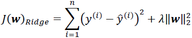
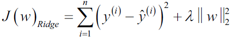
Ridge regression

regularization(e.g. L2 shrinkage or weight decay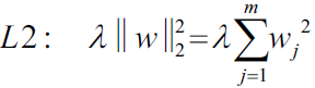) is one approach to tackling the problem of overfitting by adding additional information, and thereby shrinking the parameter values of the model to induce a penalty against complexity. The most popular approaches to regularized linear regression are the so-called Ridge Regression, least absolute shrinkage and selection operator (LASSO), and elastic Net.

The ridge regression, or L2 regularization(ℓ2 norm), addresses some of the problems of OLS regression by imposing a penalty on the size of the coefficients. Ridge Regression is an L2 penalized model where we simply add a regularization term to our least-squares cost function. This forces the learning algorithm to not only fit the data but also keep the model weights as small as possible. Note that the regularization term should only be added to the cost function during training. Once the model is trained, you want to evaluate the model’s performance using the unregularized performance measure:
OROR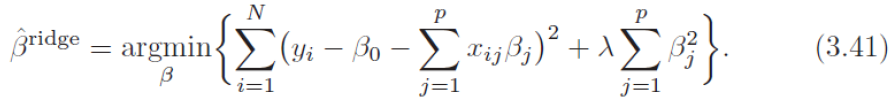
Here, the α or 𝜆 parameter is expected to be a positive value that controls the amount of shrinkage. Larger values of alpha give greater shrinkage, making the coefficients more robust to collinearity.

n instances ==>

$\large J(w)_{Ridge} = \sum_{i=1}^{m} ( y^{(i)} - \hat{y}^{(i)} )^2 + \alpha \lambda \left \| \theta \right \|^{2}_{2}$ m instances

Ridge gradient vector :

The penalty term without using the term for convenient computation

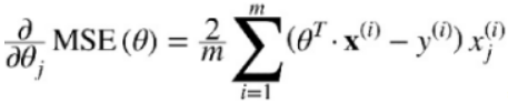
For Gradient Descent, just add 2αw to the MSE gradient vector (Equation 4-6, n features, m instances).

+αw (or +α)
αw

Note: here ==

By increasing the value of hyperparameter α or 𝜆 , we increase the regularization strength and thereby shrink the weights of our model. Please note that we don't regularize the intercept term, $\large \beta_0$ or $\large w_0$ . The hyperparameter 𝜆 controls how much you want to regularize the model. If 𝜆= 0 then Ridge Regression is just Linear Regression. If 𝜆 is very large, then all weights end up very close to zero and the result is a flat line going through the data’s mean.https://scikit-learn.org/stable/auto_examples/linear_model/plot_ridge_path.html

import numpy as np
import matplotlib.pyplot as plt
from sklearn import linear_model

# X is the 10x10 Hilbert matrix
X = 1.0 / (np.arange(1, 11) + np.arange(0, 10)[:, np.newaxis])
y = np.ones(10)

n_alphas = 200
alphas = np.logspace(-10, -2, n_alphas)

coefs = []
for a in alphas:
    ridge = linear_model.Ridge(alpha=a, fit_intercept=False)
    ridge.fit(X, y)
    coefs.append(ridge.coef_)
    
ax = plt.gca()

ax.plot(alphas, coefs)
ax.set_xscale("log")
ax.set_xlim(ax.get_xlim()[::-1])  # reverse axis
plt.xlabel("alpha")
plt.ylabel("weights")
plt.title("Ridge coefficients as a function of the regularization")
plt.axis("tight")
plt.show()

将 (3.41) 的准则写成矩阵形式
可以简单地看出岭回归的解为（本质在自变量信息矩阵的主对角线元素上人为地加入一个非负因子(Ridge Regression closed-form solution)

from sklearn.pipeline import Pipeline
from sklearn.preprocessing import StandardScaler
from sklearn.preprocessing import PolynomialFeatures

np.random.seed(42)
m=20 #number of instances
X= 3*np.random.rand(m,1) #one feature  #X=range(0,3)
              #noise
y=1 + 0.5*X + np.random.randn(m,1)/1.5 
X_new = np.linspace(0,3, 100).reshape(100,1)
 
from sklearn.linear_model import Ridge
 
def plot_model(model_class, polynomial, alphas, **model_kargs):
    for alpha, style in zip( alphas, ("b-", "y--", "r:") ):
        model = model_class(alpha, **model_kargs) if alpha>0 else LinearRegression()
        if polynomial:
            model = Pipeline([
                ("poly_features", PolynomialFeatures(degree=10, include_bias=False)),
                ("std_scaler", StandardScaler()),
                ("regul_reg", model) #regulized regression
            ])
        model.fit(X,y)
        y_new_regul = model.predict(X_new)
        lw = 5 if alpha>0 else 1
        plt.plot(X_new, y_new_regul, style, linewidth=lw, label=r"$\alpha = {}$".format(alpha) )
    plt.plot(X,y, "b.", linewidth=3)
    plt.legend(loc="upper left", fontsize=15)
    plt.xlabel("$x_1$", fontsize=18)
    plt.axis([0,3, 0,4])
 
plt.figure(figsize=(8,4) )
plt.subplot(121)
plot_model(Ridge, polynomial=False, alphas=(0,10,100), random_state=42)#plain Ridge models are used, leading to 
plt.ylabel("$y$", rotation=0, fontsize=18)
 
plt.subplot(122)
plot_model(Ridge, polynomial=True, alphas=(0,10**-5, 1), random_state=42)
plt.title("Figure 4-17. Ridge Regression")
plt.show()

If α =0 or 𝜆=0 then Ridge Regression is just Linear Regression.
If α is very large, then all weights end up very close to zero and the result is a flat line going through the data’s mean

Figure 4-17 shows several Ridge models trained on some linear data using different α value. On the left, plain Ridge models are used, leading to linear predictions. On the right, the data is first expanded using PolynomialFeatures(degree=10), then it is scaled using a StandardScaler, and finally the Ridge models are applied to the resulting features: this is Polynomial Regression with Ridge regularization. Note how increasing α leads to flatter (i.e., less extreme, more reasonable) predictions; this reduces the model’s variance but increases its bias.

The Ridge class of the sklearn.linear_model module implements ridge regression. To implement this model, create a class named RidgeRegressionModel that extends the LinearRegressionModel class, and run the following code:

In the new class, the get_model() method is overridden to return the ridge regression model of scikit-learn while reusing the other methods in the parent class. The alpha value is set to 0.5, and the rest of the model parameters are left as defaults. The ridge_reg_model variable represents an instance of our ridge regression model, and the learn() command is run with the usual parameters values.

from sklearn.linear_model import Ridge

class RidgeRegressionModel(LinearRegressionModel):        
    def get_model(self):
        return Ridge( alpha=.5 )
    
ridge_reg_model = RidgeRegressionModel()
ridge_reg_model.learn( df_x, jpm_prices,
                       start_date='2018', end_date='2019',
                       lookback_period=20
                     )

%matplotlib inline
import matplotlib.pyplot as plt

ridge_reg_model.df_result.plot( title='JPM prediction by OLS',
                                style=['b-', 'g--'],
                                figsize=(12,8),
                              )
plt.show()

ridge_reg_model.df_result

Create a function called print_regression_metrics() to print the various risk metrics covered earlier:

from sklearn.metrics import ( mean_absolute_error,
                              mean_squared_error,
                              explained_variance_score,
                              r2_score
                            )

def print_regression_metrics( df_result ):
    # convert the pandas.core.series.Series object to a list object
    actual = list( df_result['Actual'] )
    predicted = list( df_result['Predicted'] )
    
    print( 'Mean Absolute Error:',
           mean_absolute_error(actual, predicted) 
         )
    print( 'mean_squared_error:', 
           mean_squared_error(actual, predicted)
         )
    print( 'explained_variance_score:', 
            explained_variance_score(actual, predicted)
         )
    print( 'r2_score:',
           r2_score(actual, predicted)
         )
    
print_regression_metrics( ridge_reg_model. df_result )

Both Mean Error scores(MAE and MSE) of the ridge regression model are lower than the linear regression model and are closer to zero. The explained variance score and the $\large R^2$ score are higher than the linear regression model and are closer to 1. This indicates that our ridge regression model is doing a better job of prediction than the linear regression model. Besides having better performance, ridge regression computations are less costly than the original linear regression model.

Selecting meaningful features

If we notice that a model performs much better on a training dataset than on the test dataset, this observation is a strong indicator of overfitting. overfitting means the model fits the parameters too closely with regard to the particular observations in the training dataset, but does not generalize well to new data, and we say the model has a high variance. The reason for the overfitting is that our model is too complex for the given training data. Common solutions to reduce the generalization error are listed as follows:

Collect more training data
Introduce a penalty for complexity via regularization
Choose a simpler model with fewer parameters
Reduce the dimensionality of the data

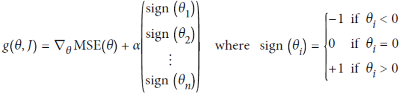
L1 and L2 regularization as penalties against model complexity

We recall from cp3 A Tour of ML Classifiers_stratify_bincount_likelihood_logistic regression_odds ratio_decay_L2 scikitlearnhttps://blog.csdn.net/Linli522362242/article/details/96480059, that L2 regularization is one approach to reduce the complexity of a model by penalizing large individual weights, where we defined the L2 norm of our weight vector w as follows:

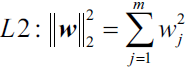
Another approach to reduce the model complexity is the related L1 regularization: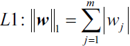

Here, we simply replaced the square of the weights by the sum of the absolute values of the weights. In contrast to L2 regularization, L1 regularization usually yields sparse[spɑrs] feature vectors; most feature weights will be zero. Sparsity['spɑ:sɪtɪ] can be useful in practice if we have a high-dimensional dataset with many features that are irrelevant[ɪˈreləvənt] especially cases where we have more irrelevant dimensions than samples. In this sense, L1 regularization can be understood as a technique for feature selection.

A geometric interpretation of L2 regularization and L1 regularization

As mentioned in the previous section, L2 regularization adds a penalty term to the cost function that effectively results in less extreme weight values compared to a model trained with an unregularized cost function. To better understand how L1 regularization encourages sparsity, let's take a step back and take a look at a geometric interpretation of regularization. Let us plot the contours of a convex cost function for two weight coefficients and . Here, we will consider the Sum of Squared Errors (SSE) cost function that we used for Adaline in https://blog.csdn.net/Linli522362242/article/details/96429442, Training Simple Machine Learning Algorithms for Classification, since it is spherical [ˈsfɪrɪkəl, ˈsfɛr-] and easier to draw than the cost function of logistic regression; however, the same concepts apply to the latter. Remember that our goal is to find the combination of weight coefficients that minimize the cost function for the training data, as shown in the following figure (the point in the center of the ellipses):

Now, we can think of regularization as adding a penalty term $\large \lambda \left \| w \right \|_{2}^{2}$ to the cost function to encourage smaller weights; or, in other words, we penalize large weights.

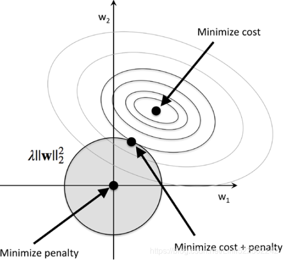
Thus, by increasing the regularization strength via the regularization parameter , we shrink the weights towards zero and decrease the dependence of our model on the training data. Let's illustrate this concept in the following figure for the L2 penalty term.
04_TrainingModels_02_regularization_L2_cost_Ridge_Lasso_Elastic Net_Early Stopping: https://blog.csdn.net/Linli522362242/article/details/104070847
The quadratic L2 regularization term is represented by the shaded ball. Here, our weight coefficients cannot exceed our regularization budget—the combination of the weight coefficients###W=w1, w2, w3...wn### cannot fall outside the shaded area. On the other hand, we still want to minimize the cost function(such asThe term is just added for our convenience https://blog.csdn.net/Linli522362242/article/details/96480059). Under the penalty constraint, our best effort is to choose the point where the L2 ball intersects with the contours of the unpenalized cost function. The larger the value of the regularization parameter gets, the faster the penalized cost function grows, which leads to a narrower L2 ball. For example, if we increase the regularization parameter towards infinity, the weight coefficients will become effectively zero, denoted by the center of the L2 ball. To summarize the main message of the example: our goal is to minimize the sum of the unpenalized cost function plus the penalty term $\large \lambda \left \| w \right \|_{2}^{2}$ , which can be understood as adding bias and preferring a simpler model to reduce the variance(try to underfit) in the absence of sufficient training data to fit the model.

Now let's discuss L1 regularization and sparsity. The main concept behind L1 regularization is similar to what we have discussed here. However, since the L1 penalty is the sum of the absolute weight coefficients (remember that the L2 term is quadratic), we can represent it as a diamond shape budget, as shown in the following figure:

In the preceding figure, we can see that the contour of the cost function touches the L1 diamond at . Since the contours of an L1 regularized system are sharp, it is more likely that the optimum—that is, the intersection between the ellipses of the cost function and the boundary of the L1 diamond—is located on the axes, which encourages sparsity. The mathematical details of why L1 regularization can lead to sparse solutions are beyond the scope of this book. If you are interested, an excellent section on L2 versus L1 regularization can be found in section 3.4 of The Elements of Statistical Learning, Trevor Hastie, Robert Tibshirani, and Jerome Friedman, Springer.

Other regression models

The sklearn.linear_model module contains various regression models that we can consider implementing in our model. The remaining sections briefly describe them. A full list of linear models is available at 1.1. Linear Models — scikit-learn 1.1.2 documentation

Lasso regression

Similar to ridge regression, Least Absolute Shrinkage and Selection Operator (LASSO) regression is also another form of regularization that involves penalizing the sum of absolute values of regression coefficients. It uses the L1 regularization(ℓ1 norm) technique. The cost function for the LASSO regression can be written as follows:
OR
Like ridge regression, the alpha parameter α controls the strength of the penalty. However, for geometric reasons, LASSO regression produces different results than ridge regression since it forces a majority of the coefficients to be set to zero. It is better suited for estimating sparse coefficients and models with fewer parameter values.

Figure 4-18 shows the same thing as Figure 4-17 but replaces Ridge models with Lasso models and uses smaller α values.

from sklearn.linear_model import Lasso

from sklearn.pipeline import Pipeline
from sklearn.preprocessing import StandardScaler
from sklearn.preprocessing import PolynomialFeatures

np.random.seed(42)
m=20 #number of instances
X= 3*np.random.rand(m,1) #one feature  #X=range(0,3)
              #noise
y=1 + 0.5*X + np.random.randn(m,1)/1.5 
X_new = np.linspace(0,3, 100).reshape(100,1)
 
from sklearn.linear_model import Ridge
 
def plot_model(model_class, polynomial, alphas, **model_kargs):
    for (alpha, style) in zip( alphas, ("b-", "y--", "r:") ):
        model = model_class(alpha, **model_kargs) if alpha>0 else LinearRegression()

        if polynomial:
            model = Pipeline([
                ("poly_features", PolynomialFeatures(degree=10, include_bias=False)),
                ("std_scaler", StandardScaler()),
                ("regul_reg", model) #regulized regression
            ])
        model.fit(X,y)
        y_new_regul = model.predict(X_new)
        lw = 5 if alpha>0 else 1
        plt.plot(X_new, y_new_regul, style, linewidth=lw, label=r"$\alpha = {}$".format(alpha) )
    plt.plot(X,y, "b.", linewidth=3)
    plt.legend(loc="upper left", fontsize=15)
    plt.xlabel("$x_1$", fontsize=18)
    plt.axis([0,3, 0,4])

plt.figure(figsize=(8,4))
plt.subplot(121)
plot_model(Lasso, polynomial=False, alphas=(0, 0.1, 1), random_state=42)
plt.ylabel("$y$", rotation=0, fontsize=18)
 
plt.subplot(122)
plot_model(Lasso, polynomial=True, alphas=(0, 10**-7, 1), random_state=42)
plt.title("Figure 4-18. Lasso Regression")
plt.show()

An important characteristic of Lasso Regression is that it tends to completely eliminate the weights of the least important features最不重要 (i.e., set them to zero). For example, the dashed line in the right plot on Figure 4-18 (with α = $\large 10^{-7}$ ) looks quadratic, almost linear(compared to Figure 4-17 ):since all the weights for the high-degree polynomial features are equal to zero. In other words, Lasso Regression automatically performs feature selection and outputs a sparse model (i.e., with few nonzero feature weights).
==>

Lasso gradient vector:

Note: here ==

from sklearn.linear_model import Lasso

class LassoRegressionModel(LinearRegressionModel):        
    def get_model(self):
        return Lasso( alpha=.5 )
    
lasso_reg_model = LassoRegressionModel()
lasso_reg_model.learn( df_x, jpm_prices,
                       start_date='2018', end_date='2019',
                       lookback_period=20
                     )

%matplotlib inline
import matplotlib.pyplot as plt

lasso_reg_model.df_result.plot( title='JPM prediction by OLS',
                                style=['b-', 'g--'],
                                figsize=(12,8),
                              )
plt.show()

Elastic net

Elastic net is another regularized regression method that combines the L1 and L2 penalties of the LASSO and ridge regression methods. The cost function for elastic net can be written as follows: https://blog.csdn.net/Linli522362242/article/details/104070847

OR Note: is for convenient computation

The alpha values are explained here:

Here, alpha and l1_ratio are parameters of the ElasticNet function.

When alpha is 0, the cost function is equivalent to an OLS( or $\large MSE(\theta)$ ).
When l1_ratio is 0, the penalty is a ridge or L2 penalty.
When l1_ratio is 1, the penalty is a LASSO or L1 penalty.
When l1_ratio is between 0 and 1, the penalty is a combination of L1 and L2.

So when should you use plain Linear Regression (i.e., without any regularization), Ridge, Lasso, or Elastic Net? It is almost always preferable to have at least a little bit of regularization, so generally you should avoid plain Linear Regression. Ridge is a good default, but if you suspect怀疑 that only a few features are actually useful, you should prefer Lasso or Elastic Net since they tend to reduce the useless features’ weights down to zero as we have discussed. In general, Elastic Net is preferred over Lasso since Lasso may behave erratically不规律地 when the number of features is greater than the number of training instances or when several features are strongly correlated.

from sklearn.linear_model import ElasticNet

class ElasticNetRegressionModel(LinearRegressionModel):        
    def get_model(self):
        return ElasticNet( alpha=.5 )
    
elasticNet_reg_model = ElasticNetRegressionModel()
elasticNet_reg_model.learn( df_x, jpm_prices,
                            start_date='2018', end_date='2019',
                            lookback_period=20
                          )

%matplotlib inline
import matplotlib.pyplot as plt

elasticNet_reg_model.df_result.plot( title='JPM prediction by OLS',
                                style=['b-', 'g--'],
                                figsize=(12,8),
                              )
plt.show()

The ElasticNet class of sklearn.linear_model implements elastic net regression.

Conclusion

We used a single-asset, trend-following momentum strategy
(Momentum, also referred to as MOM, is an important measure of speed and magnitude of price moves.https://blog.csdn.net/Linli522362242/article/details/126443770

trend-following:https://blog.csdn.net/Linli522362242/article/details/121896073

https://blog.csdn.net/Linli522362242/article/details/126353102

) by regression to predict the prices of JPM(J.P. Morgan) using GS(Goldman Sachs (GS)), with the assumption that the pair is cointegrated and highly correlated. We can also consider cross-asset momentum to obtain better results from diversification. The next section explores multi-asset regression for predicting security returns.

Predicting returns with a cross-asset momentum model

In this section, we will create a cross-asset momentum model by having the prices of four diversified assets predict the returns of JPM on a daily basis for the year of 2018. The prior 1-month, 3-month, 6-month, and 1-year of lagged returns of the S&P 500 stock index, 10-year treasury bond index, US dollar index, and gold prices will be used for fitting our model. This gives us a total of 16 features. Let's begin by preparing our datasets for developing our models.

(使用4个tickers形成的16个特征值(df_lagged)的连续多个之前日期的adjusted closing prices作为样本训练当前日期的model，使用该模型对当前的jpm closing price进行预测。每个日期都有一个model对该日期进行预测jpm closing price)

Preparing the independent variables

The ticker symbol for the S&P 500 stock index is SPX. We will use the SPDR Gold Trust (ticker symbol: GLD) to denote a share of the gold bullion/ˈbʊliən/金银 as a proxy for gold prices. The Invesco DB US Dollar Index Bullish/ˈbʊlɪʃ/看涨的 Fund (ticker symbol: UUP) will proxy the US dollar index. The iShares 7-10 Year Treasury Bond ETF (ticker symbol: IEF) will proxy the 10-year Treasury Bond Index. Run the following code to download our datasets:

# ^GSPC : SPX
# https://blog.csdn.net/Linli522362242/article/details/126269188
symbol_list = ['^GSPC','GLD','UUP','IEF']

symbols = ' '.join(symbol_list)
symbols

import yfinance as yf

df = yf.download( symbols)
df

Combine the adjusted closing prices into a single pandas DataFrame named df_assets with the following codes and remove empty values with the dropna() command:

df_assets=df['Adj Close'].dropna()
df_assets

from statsmodels.tsa.stattools import coint

for tick in symbol_list:
    x = df_assets[tick].loc['2008-02-29':].dropna()
    y = jpm_prices.loc['2008-02-29':].dropna().values
    cm = np.corrcoef(  x,
                       y
                    )
    print('ticker:', tick)
    print('correlation coefficient:', cm[0,1])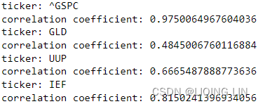

Proved correlation!

Calculate the lagged percentage returns of our df_assets dataset with the following code:

On average, the number of trading days in a month is 21 days for the U.S market, but the number varies from month to month. For example, in 2021, January and February have 19 trading days, while March has 23 trading days, which is the most for any month.

On average, the number of trading days in a year is 252 days, which translates to 21 trading days on average each month and 63 trading days per quarter.
https://therobusttrader.com/how-many-trading-days-in-a-year/#:~:text=On%20average%2C%20the%20number%20of,63%20trading%20days%20per%20quarter.

# df_assets.columns : Index(['GLD', 'IEF', 'UUP', '^GSPC'], dtype='object')
# pct_change() : prices-prices.shift(1)/prices.shift(1)
# pct_change() : the percentage change over the prior period values
df_assets_1m = df_assets.pct_change( periods=21 )
df_assets_1m.columns = [ '%s_1m' % col 
                         for col in df_assets.columns
                       ]
df_assets_3m = df_assets.pct_change( periods=63 )
df_assets_3m.columns = [ '%s_3m' % col
                         for col in df_assets.columns
                       ]
df_assets_6m = df_assets.pct_change( periods=126 )
df_assets_6m.columns = [ '%s_6m' % col
                         for col in df_assets.columns
                       ]
df_assets_12m = df_assets.pct_change( periods=252 )
df_assets_12m.columns = [ '%s_12m' % col
                          for col in df_assets.columns
                        ]
df_assets_1m

Time series objects cannot be directly normalized（Otherwise, trend changes cannot be captured）, here we have done a certain degree of normalization using pct_change()
In the pct_change() command, the periods parameter specifies the number of periods to shift. We assumed 21 trading days in a month when calculating the lagged returns. Combine the four pandas DataFrame objects into a single DataFrame with the join() command:

df_lagged = df_assets_1m.join( df_assets_3m )\
                        .join( df_assets_6m )\
                        .join( df_assets_12m ).dropna()
df_lagged

Use the info() command to view its properties:

df_lagged.info()

The output is truncated, but you can see 16 features as our independent variables spanning the years 2008 to 2022. Let's continue to obtain the dataset for our target variables.

Preparing the target variables

The closing prices of JPM having been downloaded to the pandas Series object jpm_prices earlier, simply calculate the actual percentage returns with the following code:

jpm_prices = yf.download( 'JPM' )['Adj Close']
jpm_prices

y = jpm_prices.pct_change().loc['2008-02-29':]
y

We obtain a pandas Series object as our target variable y.

A multi-asset linear regression model

In the previous section, we used a single asset with the prices of GS for fitting our linear regression model. This same model, LinearRegressionModel, accommodates multiple assets(one instace martrix: 16 features x lookback_period ==> W [lookback_period x 16 features] in linear model). Run the following commands to create an instance of this model and use our new datasets:

# from sklearn.linear_model import LinearRegression

# class LinearRegressionModel(object):
#     def __init__(self):
#         self.df_result = pd.DataFrame(columns=['Actual', 'Predicted'])

#     def get_model(self):
#         return LinearRegression(fit_intercept=False)

#     def learn(self, df, ys, start_date, end_date, lookback_period=20):
#         model = self.get_model()
        
#         df.sort_index(inplace=True)
#         for date in df[start_date:end_date].index:
#             # Fit the model
#             x = self.get_prices_since(df, date, lookback_period)
#             y = self.get_prices_since(ys, date, lookback_period)
#             model.fit(x.values, y.ravel())

#             # Predict the current period
#             x_current = df.loc[date].values
#             [y_pred] = model.predict([x_current])

#             # Store predictions
#             new_index = pd.to_datetime(date, format='%Y-%m-%d')
#             y_actual = ys.loc[date]
#             self.df_result.loc[new_index] = [y_actual, y_pred]

#     def get_prices_since(self, df, date_since, lookback):
#         index = df.index.get_loc(date_since)
#         return df.iloc[index-lookback:index]

multi_linear_model = LinearRegressionModel()
multi_linear_model.learn( df_lagged, y, 
                          start_date='2018',
                          end_date='2019',
                          lookback_period=10
                        )
multi_linear_model.df_result

In the linear regression model instance, multi_linear_model , the learn() command is supplied with the df_lagged dataset with 16 features and y as the percentage changes of JPM. The lookback_period value is reduced in consideration of the limited lagged returns data available. Let's plot the actual versus predicted percentage changes of JPM:

multi_linear_model.df_result.plot( title='JPM actual versus predicted percentage returns',
                                   style=['-', '--'], 
                                   figsize=(12,8)
                                 )
plt.show()

This would give us the following graph in which the solid lines show the actual percentage returns of JPM, while the dotted lines show the predicted percentage returns:

(此外也 Proved there is a cointegration in daily price change : 一直围绕均值0波动。而均值不随时间变化; 如果两组序列是非平稳的，但它们的线性组合可以得到一个平稳序列，那么我们就说这两组时间序列数据具有协整的性质，我们同样可以把统计性质用到这个组合的序列上来)

How well did our model perform? Let's run the same performance metrics in the print_regression_metrics() function defined in the previous section:

print_regression_metrics( multi_linear_model.df_result )

The explained variance score and $\large R^2$ scores are in the negative range, suggesting that the model performs below average. Can we perform better? Let's explore more complex tree models used in regression.

A $\large R^2 < 0$ score indicates that the prediction performs below average.
Negative values mean that the model fits worse than the baseline model. Models with negative values usually indicate issues in the training data or process and cannot be used.
But the performance issue here is not because of the preprocessing of the training data, but because we use a linear model
########## Proved : Don't do it

from sklearn.preprocessing import MinMaxScaler

mms = MinMaxScaler()
df_lagged_mms = pd.DataFrame( mms.fit_transform( df_lagged ) )
df_lagged_mms.columns = df_lagged.columns
df_lagged_mms.index = df_lagged.index

multi_linear_model_mms = LinearRegressionModel()
multi_linear_model_mms.learn( df_lagged_mms, y, 
                              start_date='2018',
                              end_date='2019',
                              lookback_period=10
                            )

multi_linear_model_mms.df_result.plot( title='JPM actual versus predicted percentage returns',
                                       style=['-', '--'], 
                                       figsize=(12,8)
                                     )
plt.show()

print_regression_metrics( multi_linear_model_mms.df_result )

########## Don't do it

Learning with ensembles

Suppose you ask a complex question to thousands of random people, then aggregate their answers. In many cases you will find that this aggregated answer is better than an expert's answer. This is called the wisdom智慧 of the crowd. Similarly, if you aggregate the predictions of a group of predictors (such as classifiers or regressors), you will often get better predictions(more accurate and robust) than with the best individual predictor. A group of predictors is called an ensemble; thus, this technique is called Ensemble Learning, and an Ensemble Learning algorithm is called an Ensemble method.

we will focus on the most popular ensemble methods that use the majority voting principle. Majority voting simply means that we select the class label that has been predicted by the majority of classifiers, that is, received more than 50 percent of the votes. Strictly speaking, the term "majority vote" refers to binary class settings only. However, it is easy to generalize the majority voting principle to multiclass settings, which is called plurality voting. Here, we select the class label that received the most votes (the mode). The following diagram illustrates the concept of majority and plurality voting for an ensemble of 10 classifiers, where each unique symbol (triangle, square, and circle) represents a unique class label:
==

Using the training dataset, we start by training m different classifiers ( ). Depending on the technique, the ensemble can

be built from different classification algorithms(This increases the chance that they will make very different types of errors, improving the ensemble's accuracy.), for example, decision trees, support vector machines, logistic regression classifiers, and so on. Figure 7-1. Training diverse classifiers Figure
Alternatively, we can also use the same base classification algorithm, fitting different subsets of the training dataset. One prominent example of this approach is the random forest algorithm, which combines different decision tree classifiers.
The following figure illustrates the concept of a general ensemble approach using majority voting ( This majority-vote classifier is called a called hard voting classifier):
<==>

To predict a class label via simple majority or plurality voting, we can combine the predicted class labels of each individual classifier, $\large C_j$ , and select the class label, $\large \hat{y}$ , that received the most votes:

(In statistics, the mode is the most frequent event or result in a set. For example, mode{1, 2, 1, 1, 2, 4, 5, 4} = 1.)

For example, in a binary classification task where $\large class_1 = -1$ and $\large class_2=+1$ , we can write the majority vote prediction as follows:

To illustrate why ensemble methods can work better than individual classifiers alone, let's apply the simple concepts of combinatorics/ˌkɒmbɪnəˈtɒrɪks /组合学. For the following example, we will make the assumption that all n-base classifiers for a binary classification task have an equal error rate, 𝜀 . Furthermore, we will assume that the classifiers are independent and the error rates are not correlated
( if all classifiers trained on the same data that will make correlated errors. These classifiers are likely to make the same types of errors, so there will be many majority votes for the wrong class, reducing the ensemble's accuracy. https://blog.csdn.net/Linli522362242/article/details/104771157
).
Under those assumptions, we can simply express the error probability of an ensemble of base classifiers as a probability mass function of a binomial distribution:

概率质量函数(Probability Mass Function, PMF,离散型数据)

是离散随机变量在各特定取值上的概率
概率质量函数PMF是对离散随机变量定义的，本⾝代表该值的概率；
概率密度函数(Probability Density Function, PDF, 连续型数据)
where n is the number of trials, p is the probability of success, and N is the number of successes.

概率密度函数PDF是对连续随机变量定义的，本⾝不是概率，只有对连续随机变量的概率密度函数PDF在某区间内进⾏积分后才是概率
The cumulative distribution function (cdf) or distribution function of a random variable X of the continuous type, defined in terms of the pdf of X, is given by
Here, again, F(x) accumulates (or, more simply, cumulates) all of the probability less
than or equal to x. From the fundamental theorem of calculus, we have, for x values
for which the derivative exists, = f(x)=f(k) and we call f(x) the probability
density function (pdf) of X.

Under those assumptions, we can simply express the error probability of an ensemble of base classifiers as a probability mass function of a binomial distribution:

Here,is the binomial coefficient n choose k. In other words, we compute the probability that the prediction of the ensemble is wrong计算集成预测错误的概率. Now, let's take a look at a more concrete example of 11 base classifiers (n = 11, k=6), where each classifier has an error rate of 0.25 (𝜀 = 0.25 ):

$\large 6\leq k\leq 11$ :majority-vote (ensemble's prediction) requires at least 50% of predictors to be wrong

The binomial coefficient

The binomial coefficient refers to the number of ways we can choose subsets of k-unordered elements from a set of size n; thus, it is often called "n choose k." Since the order does not matter here, the binomial coefficient is also sometimes referred to as combination or combinatorial number, and in its unabbreviated form, it is written as follows:

Here, the symbol (!) stands for factorial—for example,
3! = 3 ∙ 2 ∙ 1 = 6 .

As you can see, the error rate of the ensemble (0.034) is much lower than the error rate of each individual classifier (0.25) if all the assumptions are met. Note that, in this simplified illustration, a 50-50 split五五分 by an even number of classifiers, n, is treated as an error, whereas this is only true half of the time. To compare such an idealistic ensemble classifier to a base classifier over a range of different base error rates, let's implement the probability mass function in Python:

from scipy.special import comb
import math
 
def ensemble_error(n_classifier, error_rate):
    # if n_classifier=11, then k_start=6
    k_start = int( math.ceil(n_classifier/2.) )
    probs = [ comb(n_classifier, k) *\
                   error_rate**k * (1-error_rate)**(n_classifier-k)
              for k in range(k_start, n_classifier+1) 
            ]
    return sum(probs)
 
ensemble_error(n_classifier=11, error_rate=0.25)

After we have implemented the ensemble_error function, we can compute the ensemble error rates for a range of different base errors from 0.0 to 1.0 to visualize the relationship between ensemble and base errors in a line graph:

import numpy as np
 
error_range = np.arange(0.0, 1.01, 0.01) # base errors from 0.0 to 1.0
ens_errors = [ ensemble_error(n_classifier=11, error_rate=error) 
               for error in error_range
             ]
 
import matplotlib.pyplot as plt
 
plt.plot(error_range, ens_errors, label="Ensemble error", lw=2)
 
plt.plot(error_range, error_range, ls='--', label="Base error", lw=2)
 
plt.xlabel('Base error')
plt.ylabel('Base/Ensemble error')
plt.legend(loc='upper left')
plt.grid(alpha=0.5)
plt.show()

As you can see in the resulting plot, the error probability of an ensemble is always better than the error of an individual base classifier, as long as the base classifiers perform better than random guessing (𝜀 < 0.5 ). Note that the y axis depicts the base error (dotted line) as well as the ensemble error (continuous line): $\large \hat{y}$

Implementing a simple majority vote classifier

The algorithm that we are going to implement in this section will allow us to combine different classification algorithms associated with individual weights for confidence. Our goal is to build a stronger meta-classifier that balances out the individual classifiers' weaknesses on a particular dataset. In more precise mathematical terms, we can write the weighted majority vote as follows:

Here, $\large \hat{y}$ is the predicted class label of the ensemble
is a weight associated with a base classifier, $\large C_j$ ;
$\large A$ is the set of unique class labels;
$\large \chi_A$ (Greek chi) is the characteristic function or indicator function, which returns 1 if the predicted class of the jth classifier matches the class label i ( $\large C_j(x) = i$ and ). For equal weights, we can simplify this equation and write it as follows:

To better understand the concept of weighting, we will now take a look at a more concrete example. Let's assume that we have an ensemble of three(m=3) base classifiers,, and we want to predict the class label,, of a given example, x. Two out of three base classifiers predict the class label $\large 0$ , and one, $\large C_3$ , predicts that the example belongs to class $\large 1$ .

If we weight the predictions of each base classifier equally, the majority vote predicts that the example belongs to class $\large 0$ :
Now, let's assign a weight of 0.6 to , and
let's weight and by a coefficient of 0.2:predicts that the example belongs to class 1
More simply, since 3 × 0.2 = 0.6, we can say that the prediction made by has three times more weight than the predictions by or , which we can write as follows:

To translate the concept of the weighted majority vote into Python code, we can use NumPy's convenient argmax and bincount functions:

         # np.bincount( [0,0,1], weights=[0.2,0.2,0.6] ) ==> array([0.4, 0.6])
np.argmax(np.bincount([0,0,1], weights = [0.2,0.2,0.6]))

As you will remember from the discussion on logistic regression in Cp3, A Tour of Machine Learning Classifiers Using scikit-learn
https://blog.csdn.net/Linli522362242/article/details/96480059, certain classifiers in scikit-learn can also return the probability of a predicted class label via the predict_proba method. Using the predicted class probabilities instead of the class labels for majority voting can be useful if the classifiers in our ensemble are well calibrated['kælɪbreɪtɪd]校准. The modified version of the majority vote for predicting class labels from probabilities can be written as follows:
Here, $\large p_{ij}$ is the predicted probability of the jth classifier for class label i.

To continue with our previous example, let's assume that we have a binary classification problem with class labels 𝑖 ∈ {0, 1} or and an ensemble of three classifiers .and Let's assume that the classifiersreturn the following class membership probabilities for a particular example, $\large x$ :

Using the same weights as previously (0.2, 0.2, and 0.6), we can then calculate the individual class probabilities as follows:

To implement the weighted majority vote based on class probabilities, we can again make use of NumPy, using np.average and np.argmax:

# class membership probabilities
#   class label '0', '1'
ex = np.array([[0.9, 0.1], # *0.2
               [0.8, 0.2], # *0.2
               [0.4, 0.6]  # *0.6
              ])
 
# OR # if weights not None, ex.T.dot( [0.2,0.2,0.6] ) ==> array([0.58, 0.42])
#    # if weights=None, ex.T.dot( [1,1,1] )/3 ==> array([0.7, 0.3])
    # np.average( ex, axis=0, weights=None)   ==> array([0.7, 0.3])
p = np.average( ex, axis=0, weights=[0.2,0.2,0.6]) #default weights=None
p

np.argmax(p)

# class label i= 0

Putting everything together, let's now implement MajorityVoteClassifier in Python:

I've added a lot of comments to the code to explain the individual parts. However, before we implement the remaining methods, let's take a quick break and discuss some of the code that may look confusing at first. We used the BaseEstimator and ClassifierMixin parent classes to get some base functionality for free, including the get_params and set_params methods to set and return the classifier's parameters, as well as the score method to calculate the prediction accuracy.

from sklearn.base import BaseEstimator
from sklearn.base import ClassifierMixin
from sklearn.preprocessing import LabelEncoder
from sklearn.base import clone
from sklearn.pipeline import _name_estimators
import numpy as np
import operator
 
class MajorityVoteClassifier(BaseEstimator, ClassifierMixin):
    """ A majority vote ensemble classifier
    Parameters
    ----------
    classifiers : array-like, shape = [n_classifiers]
      Different classifiers for the ensemble
    vote : str, {'classlabel', 'probability'} (default='classlabel')
      If 'classlabel' the prediction is based on the argmax of
        class labels. 
      Else if 'probability', the argmax of
        the sum of probabilities is used to predict the class label
        (recommended for calibrated classifiers).
    weights : array-like, shape = [n_classifiers], optional (default=None)
      If a list of `int` or `float` values are provided, the classifiers
      are weighted by importance; 
      Uses uniform weights if `weights=None`.
    """
    def __init__(self, classifiers, vote='classlabel', weights=None):
        self.classifiers = classifiers
        # estimators = ['a', 'a', 'b' ]
        # _name_estimators(estimators) #  [('a-1', 'a'), ('a-2', 'a'), ('b', 'b')]
        self.named_classifiers = { key:value 
                                   for key,value in _name_estimators(classifiers)
                                 }
        self.vote = vote
        self.weights = weights
    
    def fit(self, X, y):
        """ Fit classifiers.
        Parameters
        ----------
        X : {array-like, density matrix}, shape = [n_examples, n_features]
            Matrix of training examples.
        y : array-like, shape = [n_examples]
            Vector of target class labels.
        Returns
        -------
        self : object
        """
        if self.vote not in ('probability', 'classlabel'):
            raise ValueError("vote must be 'probability' or 'classlabel'"
                             "; got (vote=%r)" % self.vote
                            ) 
            # %r是一个万能的格式付，它会将后面给的参数原样打印出来，带有类型信息。
        
        if self.weights and len(self.weights)!=len(self.classifiers):
            raise ValueError("Number of classifiers and weights must be equal"
                             "; got %d num_weights, %d num_classifier"
                             % ( len(self.weights), len(self.classifiers) )
                            )
            
        # Use LabelEncoder to ensure class labels(indices) start with 0, which
        # is important for np.argmax call in self.predict
        self.labelEncoder_ = LabelEncoder()
        self.labelEncoder_.fit(y)
        self.classes_ = self.labelEncoder_.classes_ # ==> y_label_indices of set(y)
        # for examples
        # le = preprocessing.LabelEncoder()
        # le.fit([1, 2, 2, 6]) ==> LabelEncoder()
        # le.classes_ ==> array([1, 2, 6])
        # le.transform([1, 1, 2, 6]) ==> array([0, 0, 1, 2]...)
        # le.inverse_transform([0, 0, 1, 2]) ==> array([1, 1, 2, 6])
        self.classifiers_ = [] # fitted classifiers
        for clf in self.classifiers:
            # Clone does a deep copy of the model in an estimator without actually copying 
            # attached data. It yields a new estimator with the "same parameters" that has not 
            # been fit on any data.
            fitted_clf = clone(clf).fit( X, self.labelEncoder_.transform(y) ) # training
            self.classifiers_.append(fitted_clf)
        return self

Next, we will add the predict method to predict the class label via a majority vote based on the class labels (hard voting) if we initialize a new MajorityVoteClassifier object with vote='classlabel'. Alternatively, we will be able to initialize the ensemble classifier with vote='probability' (This is called soft voting. It often achieves higher performance than hard voting because it gives more weight to highly confident votes.) to predict the class label based on the class membership probabilities.

Furthermore, we will also add a predict_proba method to return the averaged probabilities, which is useful when computing the receiver operating characteristic area under the curve (ROC AUC):

    def predict_proba(self, X):
        """ Predict class probabilities for X.
        Parameters
        ----------
        X : {array-like, sparse matrix}, shape = [n_examples, n_features]
            Training vectors, where n_examples is the number of examples and
            n_features is the number of features.
        Returns
        ----------
        avg_proba : array-like, shape = [n_examples, n_classes]
            Weighted average probability for each class per example.
        """
        
        probas = np.asarray([ clf.predict_proba(X)
                              for clf in self.classifiers_
                            ]) 
        # probas : shape[num_classifiers, n_examples, num_classLabels_probabilities]
        
        #along axis_0 * w, sum element_wise
        avg_proba = np.average( probas, axis=0, weights=self.weights )
        # avg_proba : shape[n_examples, num_classLabels_probabilities]
        # OR
        # probas.shape: [num_classifiers, n_examples, num_classLabels_probabilities]
        #          ==>  [n_examples, num_classLabels_probabilities, num_classifiers]
        # via #np.transpose(probas, (1,2,0))
        # why (1,2,0) since avg_proba :shape[n_examples, num_classLabels_probabilities]
#         if self.weights : # exist classifiers' weight 
#             avg_proba = np.transpose(probas, (1,2,0)).dot( self.weights ) 
#         else:
#             avg_proba = np.transpose(probas, (1,2,0)).dot( np.ones(len(self.classifiers)) )/len(self.classifiers)
        return avg_proba
    
    def predict(self, X):
        """ Predict class labels for X.
        Parameters
        ----------
        X : {array-like, Density matrix}, shape = [n_examples, n_features]
            Matrix of training examples.
        Returns
        ----------
        maj_vote : array-like, shape = [n_examples]
            Predicted class labels.
        """
        
        if self.vote =='probability':
            # self.predict_proba(X) : shape[n_examples, num_classLabels_probabilities]
            maj_vote = np.argmax( self.predict_proba(X), axis=1 ) #axis=1 : column or features
            # return a class_label_index for each new instance from X # a list
            
        else: # self.vote == 'classlabel'
            #  Collect results from clf.predict calls
            predictions = np.asarray([ clf.predict(X) 
                                       for clf in self.classifiers_
                                     ]).T
            # prediction : a class_label list for each new instance from X
            # [ num_classifiers, n_examples ].T ==> predictions.shape: [ n_examples, num_classifiers]
            maj_vote = np.apply_along_axis( lambda x: np.argmax( 
                                                         np.bincount(x, weights=self.weights) 
                                                      ), 
                                            axis=1, 
                                            arr=predictions # Input array.
                                          ) # return a list of class_label_indx
        maj_vote = self.labelEncoder_.inverse_transform(maj_vote) #decode ==> class_label
        return maj_vote
    
    def get_params(self, deep=True):
        """ Get classifier parameter names for GridSearch"""
        # sklearn.base.BaseEstimator
        #                          deep:bool, default=True
        #                               If True, will return the parameters for this estimator 
        #                               and contained subobjects that are estimators.
        if not deep:
            return super(MajorityVoteClassifier, self).get_params(deep=False)
        else:
            out = self.named_classifiers.copy()
            # for name_estimator, estimator in ...
            for name, step in self.named_classifiers.items():
                # for parameter, value_parameter in ...
                for key, value in step.get_params(deep=True).items():
                    out['%s__%s' % (name, key)]=value
            return out

Also, note that we defined our own modified version of the get_params method to use the _name_estimators function to access the parameters of individual classifiers in the ensemble; this may look a little bit complicated at first, but it will make perfect sense when we use grid search for hyperparameter tuning in later sections.

VotingClassifier in scikit-learn

Although the MajorityVoteClassifier implementation is very useful for demonstration purposes, we implemented a more sophisticated version of this majority vote classifier in scikit-learn. The ensemble classifier is available as sklearn.ensemble.VotingClassifier in scikit-learn version 0.17 and newer.

from sklearn.base import BaseEstimator
from sklearn.base import ClassifierMixin
from sklearn.preprocessing import LabelEncoder
from sklearn.base import clone
from sklearn.pipeline import _name_estimators
import numpy as np
import operator
 
class MajorityVoteClassifier(BaseEstimator, ClassifierMixin):
    """ A majority vote ensemble classifier
    Parameters
    ----------
    classifiers : array-like, shape = [n_classifiers]
      Different classifiers for the ensemble
    vote : str, {'classlabel', 'probability'} (default='classlabel')
      If 'classlabel' the prediction is based on the argmax of
        class labels. 
      Else if 'probability', the argmax of
        the sum of probabilities is used to predict the class label
        (recommended for calibrated classifiers).
    weights : array-like, shape = [n_classifiers], optional (default=None)
      If a list of `int` or `float` values are provided, the classifiers
      are weighted by importance; 
      Uses uniform weights if `weights=None`.
    """
    def __init__(self, classifiers, vote='classlabel', weights=None):
        self.classifiers = classifiers
        # estimators = ['a', 'a', 'b' ]
        # _name_estimators(estimators) #  [('a-1', 'a'), ('a-2', 'a'), ('b', 'b')]
        self.named_classifiers = { key:value 
                                   for key,value in _name_estimators(classifiers)
                                 }
        self.vote = vote
        self.weights = weights
    
    def fit(self, X, y):
        """ Fit classifiers.
        Parameters
        ----------
        X : {array-like, density matrix}, shape = [n_examples, n_features]
            Matrix of training examples.
        y : array-like, shape = [n_examples]
            Vector of target class labels.
        Returns
        -------
        self : object
        """
        if self.vote not in ('probability', 'classlabel'):
            raise ValueError("vote must be 'probability' or 'classlabel'"
                             "; got (vote=%r)" % self.vote
                            ) 
            # %r是一个万能的格式付，它会将后面给的参数原样打印出来，带有类型信息。
        
        if self.weights and len(self.weights)!=len(self.classifiers):
            raise ValueError("Number of classifiers and weights must be equal"
                             "; got %d num_weights, %d num_classifier"
                             % ( len(self.weights), len(self.classifiers) )
                            )
            
        # Use LabelEncoder to ensure class labels(indices) start with 0, which
        # is important for np.argmax call in self.predict
        self.labelEncoder_ = LabelEncoder()
        self.labelEncoder_.fit(y)
        self.classes_ = self.labelEncoder_.classes_ # ==> y_label_indices of set(y)
        # for examples
        # le = preprocessing.LabelEncoder()
        # le.fit([1, 2, 2, 6]) ==> LabelEncoder()
        # le.classes_ ==> array([1, 2, 6])
        # le.transform([1, 1, 2, 6]) ==> array([0, 0, 1, 2]...)
        # le.inverse_transform([0, 0, 1, 2]) ==> array([1, 1, 2, 6])
        self.classifiers_ = [] # fitted classifiers
        for clf in self.classifiers:
            # Clone does a deep copy of the model in an estimator without actually copying 
            # attached data. It yields a new estimator with the "same parameters" that has not 
            # been fit on any data.
            fitted_clf = clone(clf).fit( X, self.labelEncoder_.transform(y) ) # training
            self.classifiers_.append(fitted_clf)
        return self
    
    def predict_proba(self, X):
        """ Predict class probabilities for X.
        Parameters
        ----------
        X : {array-like, sparse matrix}, shape = [n_examples, n_features]
            Training vectors, where n_examples is the number of examples and
            n_features is the number of features.
        Returns
        ----------
        avg_proba : array-like, shape = [n_examples, n_classes]
            Weighted average probability for each class per example.
        """
        
        probas = np.asarray([ clf.predict_proba(X)
                              for clf in self.classifiers_
                            ]) 
        # probas : shape[num_classifiers, n_examples, num_classLabels_probabilities]
        
        #along axis_0 * w, sum element_wise
        avg_proba = np.average( probas, axis=0, weights=self.weights )
        # avg_proba : shape[n_examples, num_classLabels_probabilities]
        # OR
        # probas.shape: [num_classifiers, n_examples, num_classLabels_probabilities]
        #          ==>  [n_examples, num_classLabels_probabilities, num_classifiers]
        # via #np.transpose(probas, (1,2,0))
        # why (1,2,0) since avg_proba :shape[n_examples, num_classLabels_probabilities]
#         if self.weights : # exist classifiers' weight 
#             avg_proba = np.transpose(probas, (1,2,0)).dot( self.weights ) 
#         else:
#             avg_proba = np.transpose(probas, (1,2,0)).dot( np.ones(len(self.classifiers)) )/len(self.classifiers)
        return avg_proba
    
    def predict(self, X):
        """ Predict class labels for X.
        Parameters
        ----------
        X : {array-like, Density matrix}, shape = [n_examples, n_features]
            Matrix of training examples.
        Returns
        ----------
        maj_vote : array-like, shape = [n_examples]
            Predicted class labels.
        """
        
        if self.vote =='probability':
            # self.predict_proba(X) : shape[n_examples, num_classLabels_probabilities]
            maj_vote = np.argmax( self.predict_proba(X), axis=1 ) #axis=1 : column or features
            # return a class_label_index for each new instance from X # a list
            
        else: # self.vote == 'classlabel'
            #  Collect results from clf.predict calls
            predictions = np.asarray([ clf.predict(X) 
                                       for clf in self.classifiers_
                                     ]).T
            # prediction : a class_label list for each new instance from X
            # [ num_classifiers, n_examples ].T ==> predictions.shape: [ n_examples, num_classifiers]
            maj_vote = np.apply_along_axis( lambda x: np.argmax( 
                                                         np.bincount(x, weights=self.weights) 
                                                      ), 
                                            axis=1, 
                                            arr=predictions # Input array.
                                          ) # return a list of class_label_indx
        maj_vote = self.labelEncoder_.inverse_transform(maj_vote) #decode ==> class_label
        return maj_vote
    
    def get_params(self, deep=True):
        """ Get classifier parameter names for GridSearch"""
        # sklearn.base.BaseEstimator
        #                          deep:bool, default=True
        #                               If True, will return the parameters for this estimator 
        #                               and contained subobjects that are estimators.
        if not deep:
            return super(MajorityVoteClassifier, self).get_params(deep=False)
        else:
            out = self.named_classifiers.copy()
            # for name_estimator, estimator in ...
            for name, step in self.named_classifiers.items():
                # for parameter, value_parameter
                for key, value in step.get_params(deep=True).items():
                    out['%s__%s' % (name, key)]=value
            return out

Using the majority voting principle to make predictions

Now it is time to put the MajorityVoteClassifier that we implemented in the previous section into action. But first, let's prepare a dataset that we can test it on. Since we are already familiar with techniques to load datasets from CSV files, we will take a shortcut and load the Iris dataset from scikit-learn's datasets module. Furthermore, we will only select two features, sepal width and petal length, to make the classification task more challenging for illustration purposes. Although our MajorityVoteClassifier generalizes to multiclass problems, we will only classify flower examples from the Iris-versicolor and Iris-virginica classes, with which we will compute the ROC AUC later. The code is as follows:https://blog.csdn.net/Linli522362242/article/details/109725186

An ensemble of decision trees

Decision trees are widely used models for classification and regression tasks, much like a binary tree, where each node represents a question leading to a yes-no answer for traversing the respective left and right nodes. The goal is to get to the right answer by asking as few questions as possible.

Traversing deep down decision trees can quickly lead to overfitting of the given data, rather than inferring the overall properties of the distributions from which they are drawn. To address this issue of overfitting, the data can be split into subsets and train on different trees, each on a subset. This way, we end up with an ensemble of different decision tree models. When random subsets of the samples are drawn with replacements for prediction, this method is called bagging or bootstrap aggregation. We may or may not get consistent results across these models, but the final model obtained by averaging the bootstrapped models yields better results than using a single decision tree. Using an ensemble of randomized decision trees is known as random forests.

Let's visit some decision tree models in scikit-learn that we may consider implementing in our multi-asset regression model.

Bagging regressor

An approach is to use the same training algorithm for every predictor(e.g. classifiers), but to train them on different random subsets of the training set. When sampling is performed with replacement, this method is called bagging装袋法(short for bootstrap aggregating自助法聚合 '. When sampling is performed without replacement, it is called pasting.

In other words, both bagging and pasting allow training instances to be sampled several times across multiple predictors, but only bagging allows training instances to be sampled several times for the same predictor. This sampling and training process is represented in Figure 7-4.

<==
Figure 7-4. Pasting/bagging training set sampling and training
Once all predictors are trained, the ensemble can make a prediction for a new instance by simply aggregating the predictions of all predictors. The aggregation function is typically the statistical mode (i.e., the most frequent prediction, just like a hard voting classifier(The majority-vote classifier is called a called hard voting classifier) ) for classification, or the average for regression. Each individual predictor has a higher bias than if it were trained on the original training set, but aggregation reduces both bias and variance. Generally, the net result is that the ensemble has a similar bias but a lower variance than a single predictor trained on the original training set. In other words,

the bagging algorithm can be an effective approach to reducing the variance(~overfitting) of a model.
However, bagging is ineffective in reducing model bias, that is, models that are too simple to capture the trend in the data well.
This is why we want to perform bagging on an ensemble of classifiers with low bias, for example, unpruned decision trees.

As you can see in Figure 7-4, predictors can all be trained in parallel, via different CPU cores or even different servers. Similarly, predictions can be made in parallel. This is one of the reasons why bagging and pasting are such popular methods: they scale可扩展性 very well.

The BaggingRegressor class of sklearn.ensemble implements the bagging regressor. We can see how a bagging regressor works for multi-asset predictions of the percentage returns of JPM. The following code illustrates this

from sklearn.ensemble import BaggingRegressor

class BaggingRegressorModel( LinearRegressionModel ):
    def get_model( self ):
        return BaggingRegressor( # base_estimator =None, then the base estimator is a DecisionTreeRegressor
                                 n_estimators=20,
                                 # bootstrapbool, default=True : with replacement
                                 #                        False: without replacement
                                 random_state=0
                               )

We created a class named BaggingRegressorModel that extends LinearRegressionModel , and the get_model() method is overridden to return the bagging regressor. The n_estimators parameter specifies 20 base estimators or decision trees in the ensemble, with the random_state parameter as a seed of 0 used by the random number generator. The rest of the parameters are default values. We run this model with the same dataset.

bagging = BaggingRegressorModel()
bagging.learn( df_lagged, y, 
               start_date='2018', end_date='2019',
               lookback_period=10
             )

Run the same performance metrics and see how our model performs:

print_regression_metrics( bagging.df_result )

The MAE and MSE values indicate that an ensemble of decision trees produces fewer prediction errors than the simple linear regression model. Also, though the explained variance score and the R2 scores are negative, it indicates a better variance of data towards the mean than is offered by the simple linear regression model.

Gradient tree boosting regression model

Gradient tree boosting, or simply gradient boosting, is a technique of improving or boosting the performance of weak learners using a gradient descent procedure to minimize the differentiable loss function. Tree models, usually decision trees, are added one at a time and build the model in a stage-wise fashion, while leaving the existing trees in the model unchanged. Since gradient boosting is a greedy algorithm, it can overfit a training dataset quickly. However, it can benefit from regularization methods that penalize various parts of the algorithm and reduce overfitting to improve its performance.

Just like AdaBoost, Gradient Boosting works by sequentially adding predictors to an ensemble, each one correcting its predecessor. However, instead of tweaking the instance weights at every iteration j( note: update all sample-weights) like AdaBoost does(𝜀 = 𝒘∙ (𝒚̂ ≠ 𝒚), 1 is assigned if the prediction on that sample is incorrect and 0 is assigned otherwise; then , then and element-wise multiplication by the cross symbol ( × ) and using the updated weights for next iteration or next weak learner: = train(𝑿, 𝒚, 𝒘) .
), this method tries to fit the new predictor to the residual errors made by the previous predictor(e.g. classifiers).

Let's start understanding Gradient Boosting with a simple example, as GB challenges many data scientists in terms of understanding the working principle:

1. Initially, we fit the model on observations producing 75% accuracy and the remaining unexplained variance is captured in the error term:
2. Then we will fit another model on the error term to pull the extra explanatory component and add it to the original model, which should improve the overall accuracy:

similar to
3. Now, the model is providing 80% accuracy and the equation looks as follows:
4. We continue this method one more time to fit a model on the error2 component to extract a further explanatory component:
5. Now, model accuracy is further improved to 85% and the final model equation looks as follows:
6. Here, if we use weighted average (higher importance given to better models that
predict results with greater accuracy than others) rather than simple addition, it
will improve the results further. In fact, this is what the gradient boosting
algorithm does!

After incorporating weights, the name of the error changed from error3 to error4, as both errors may not be exactly the same. If we find better weights, we will probably get an accuracy of 90% instead of simple addition, where we have only got 85%.

Gradient boosting involves three elements:

Loss function to be optimized: Loss function depends on the type of problem being solved. In the case of
- regression problems, Mean Squared Error is used, and in
- classification problems, the logarithmic loss will be used. In boosting, at each stage, unexplained loss from prior iterations will be optimized rather than starting from scratch.
Weak learner to make predictions: Decision trees are used as a weak learner in gradient boosting.
Additive model to add weak learners to minimize the loss function: Trees are added one at a time and existing trees in the model are not changed. The gradient descent procedure is used to minimize the loss when adding trees.

The algorithm for Gradient boosting consists of the following steps:
输出是强学习器f(x)梯度提升树(GBDT)原理小结 - 刘建平Pinard - 博客园

1. Initialize model with a constant value(使损失函数极小化的常数值):
a constant functionOR
each sample from index i = 1, 2, …, N

Initializes the constant optimal constant model, which is just a single terminal node that will be utilized as a starting point to tune it further in the next steps

######
The first step is creating an initial constant value prediction .
is the loss function and suppose our loss function is squared loss in our regression case.OR
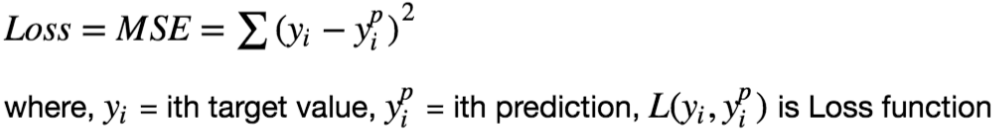
$\large argmin$ means we are searching for the value that minimizes .
Let’s compute the valueγ by using our actual loss function. To findγ that minimizes , we are taking a derivative of  with respect toγ.

And we are findingγ that makes  .
(the mean of y)
It turned out that the valueγ that minimizes  is the mean of y. So we used y mean for our initial prediction  in the last section. $\large f_0(x) = \dot{\gamma} = \bar{y}$
(The γ value obtained by different model' loss functions are different)

######
step 2. For Iteration m = 1 to M（从区域/树1 到区域/树M，逐渐产生disjoin regions）:
$\large M$ denotes the number of trees we are creating and
the small represents the index of each tree.
- a) For each sample from index i = 1, 2, …, N
  compute: 计算负梯度OR
  calculates the (so-called pseudo-residuals伪残差)residuals/errors by comparing actual outcome with predicted results
  计算损失函数的负梯度在当前模型的值，将它作为残差的估计，
  followed by (2b and 2c) in which the next decision tree will be fitted on error terms to bring in more explanatory power to the model
  (==>),
  ##########################
  We are calculating residuals by taking a derivative of the loss function with respect to the previous prediction $\large f_{m-1}$ (OR $\large F_{m-1}$ ) and multiplying it by −1. As you can see in the subscript index, is computed for each single sample i. Some of you might be wondering why we are calling this residuals. This value is actually negative gradient that gives us guidance on the directions (+/−) and the magnitude in which the loss function can be minimized. You will see why we are calling it residuals shortly. By the way, this technique where you use a gradient to minimize the loss on your model is very similar to gradient descent technique which is typically used to optimize neural networks. (In fact, they are slightly different from each other. If you are interested, please look at this article Gradient boosting performs gradient descent detailing that topic.)
  Let’s compute the residuals here. $\large f_{m-1}$ (OR $\large F_{m-1}$ ) in the equation means the prediction from the previous step. In this first iteration, it is $\large f_0$ (OR $\large F_0$ ). We are solving the equation for residuals .
  We can take 2 out of it as it is just a constant. That leaves us $\large r_{im} = y_i - F_{m-1}$ . You might now see why we call it residuals. This also gives us interesting insight that the negative gradient that provides us the direction and the magnitude to which the loss is minimized is actually just residuals.
  
  实际应用过程中可以使用一个回归树直接对数据进行拟合产生 $F_0(x)=F_m(x) + r_{im}$ OR
  In the actual application, a regression tree is used to directly fit the data to generate $F_0(x)=F_m(x) + r_{im}$ OR , note residual $r_{im}$
- To minimize these residuals $\large r_{im}$ , we are building a regression tree model with as its feature and the residuals $\large r_{im} = y_i - F_{m-1}$ as its target. The reasoning behind that is if we can find some patterns between x and $\large r_{im}$ by building the additional weak model, we can reduce the residuals by utilizing it.
  ##########################
- b) Fit a regression tree with features $\large x$ to against residuals $\large r_{im}$ and then create terminal regions $\large \mathbf{R_{jm}}$ for j = 1, 2, …, , 其中为回归区域/树m的叶子节点的个数。
  $\large j$ represents a terminal node (i.e. leave index : start from 1) in the tree,
  $\large m$ denotes the tree index, and
  capital $\large J$ means the total number of leaves.
  residual tree with features x and terminal nodes
  
  To simplify the demonstration, we are building very simple trees each of that only has 1 split and 2 terminal nodes which is called “stump”. Please note that gradient boosting trees usually have a little deeper trees(>=1) such as ones with 8 to 32 terminal nodes.
  ==> $\large J_m = 2$
- c) for j = 1, 2, …, , compute
  
  OR
  $\large f_{m-1}$ (OR $\large F_{m-1}$ ) in the equation means the prediction from the previous step
  
  We are searching for $\large \gamma_{jm}$ that minimizes the loss function on each terminal node j (叶子区域j). $\large \sum_{x_i \euro R_{jm} }^{}$ means we are aggregating the loss on all the sample $\large x_i s$ that belong to the terminal node $\large \mathbf{R_{jm}}$ . Let’s plugin the loss function into the equation.
  Then, we are finding that makes the derivative of Σ(*) equals zero.Please note that $\large n_j$ means the number of samples in the terminal node j. This means the optimal (or $\large \gamma$ ) that minimizes the loss function is the average of the residuals $\large r_{im}$ in the terminal node $\large \mathbf{R_{jm}}$ . In other words, $\large \gamma_{jm}$ is the regular prediction values of regression trees that are the average of the target values (in our case, residuals) in each terminal node.==> $\gamma_{jm} = ( \gamma_{1m}=6.0, \gamma_{2m}=-5.9 )$
- d) Update the model 更新强学习器:
  
  https://en.wikipedia.org/wiki/Gradient_boosting
  
  add the extra component to the model at last iteration
  
  ######
  In the final step, we are updating the prediction of the combined model $\large F_m$ . $\large \gamma_{jm} 1 (x\euro R_{jm})$ means that we pick the value $\large \gamma_{jm}$ if a given x falls in a terminal node $\large \mathbf{R_{jm}}$ . As all the terminal nodes are exclusive由于所有终端节点都是互斥的, any given single x falls into only a single terminal node and corresponding $\large \gamma_{jm}$ is added to the previous prediction $\large F_{m-1}$ and it makes updated prediction F𝑚.
  
  In fact, gradient boosting algorithm does not simply add to $\large F_{m-1}$ as it makes the model overfit to the training data. Instead, is scaled down by learning rate $\large v$ which ranges between 0 and 1, and then added to $\large F_{m-1}$ .
  
  $\large v$ is learning rate ranging between 0 and 1 which controls the degree of contribution of the additional tree prediction to the combined prediction F𝑚. A smaller learning rate $\large v$ reduces the effect of the additional tree prediction, but it basically also reduces the chance of the model overfitting to the training data.
  
  In this example, we use a relatively big learning rate $v = 0.9$ to make the optimization process easier to understand, but it is usually supposed to be a much smaller value such as 0.1.
  ######
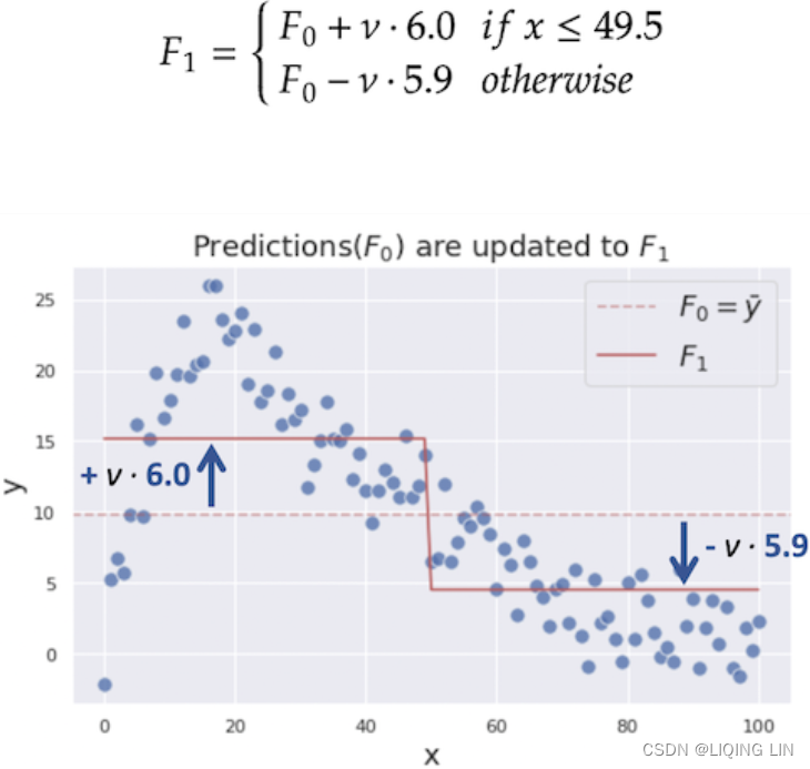
  repeat step2(a-d)
Output:
Now we have gone through the whole steps. To get the best model performance, we want to iterate step2 M times, which means adding M trees to the combined model. In reality, you might often want to add more than 100 trees to get the best model performance.

ensemble all weak learners to create a strong learner.（类似于AdaBoost (Adaptive Boosting适应性提升)）https://towardsdatascience.com/all-you-need-to-know-about-gradient-boosting-algorithm-part-1-regression-2520a34a502

The sklearn.ensemble module provides a gradient-boosting regressor called GradientBoostingRegressor https://blog.csdn.net/Linli522362242/article/details/105046444

Random forests regression

Random forests consist of multiple decision trees each based on a random sub-sample of the training data and uses averaging to improve the predictive accuracy and to control overfitting. Selection by random inadvertently introduces some form of bias. However, due to averaging, it variance also decreases, helping to compensate for the increase in bias, and is considered to yield an overall better model.

The random forest algorithm can be summarized in four simple steps:

1. Draw a random bootstrap sample of size n (randomly choose n samples from the training set with replacement).
2. Grow a decision tree from the bootstrap sample. At each node:
- a. Randomly select m features without replacement (m : the subset of total p features ).
- b. Split the node using the feature that provides the best split according to the objective function, for instance, maximizing the information gain.
3. Repeat the steps 1-2 k times(=n_estimators).
4. Aggregate the prediction by each tree to assign the class label by majority vote.

We should note one slight modification in step 2 when we are training the individual decision trees: instead of evaluating all features to determine the best split at each node, we only consider a random subset of those.

sklearn.ensemble.RandomForestClassifier — scikit-learn 1.1.2 documentation

max_features {“sqrt”, “log2”, None}, int or float, default=”sqrt”

The number of features to consider when looking for the best split:

If int, then consider max_features features at each split.
If float, then max_features is a fraction and max(1, int(max_features * n_features_in_)) features are considered at each split.
If “auto”, then max_features=sqrt(n_features). $\large m = \sqrt{p}$
If “sqrt”, then max_features=sqrt(n_features) $\large m = \sqrt{p}$ .
If “log2”, then max_features=log2(n_features).
If None, then max_features=n_features.

As we have discussed, a Random Forest is an ensemble of Decision Trees, generally trained via the bagging method (or sometimes pasting), typically with max_samples set to the size of the training set. Instead of building a BaggingClassifier and passing it a DecisionTreeClassifier, you can instead use the RandomForestClassifier class, which is more convenient and optimized for Decision Trees (similarly, there is a RandomForestRegressor class for regression tasks). The following code trains a Random Forest classifier with 500 trees (each limited to maximum 16 nodes), using all available CPU cores:

bag_clf = BaggingClassifier(                  #each limited to maximum 16 nodes   
    DecisionTreeClassifier( splitter="random", max_leaf_nodes=16, random_state=42 ),
    n_estimators= 500, 
    max_samples=1.0, #The number of samples to draw from X to train each base estimator. #max_samples * X.shape[0]
    bootstrap=True, #samples are drawn with replacement #bootstrap
    random_state=42,
    n_jobs=-1 #using all available CPU cores
)
 
bag_clf.fit(X_train, y_train)
y_pred = bag_clf.predict(X_test)

use the RandomForestClassifier class $\large m = \sqrt{p}$


from sklearn.ensemble import RandomForestClassifier
                                                   #each limited to maximum 16 nodes   #using all available CPU cores
rnd_clf = RandomForestClassifier(n_estimators=500, max_features='sqrt',
                                 max_leaf_nodes=16, random_state=42, n_jobs=-1)
 
rnd_clf.fit(X_train, y_train)
y_pred_rf = rnd_clf.predict(X_test)
 
np.sum(y_pred==y_pred_rf) / len(y_pred)  #almost identical predictions

With a few exceptions, a RandomForestClassifier has all the hyperparameters of a DecisionTreeClassifier (to control how trees are grown), plus all the hyperparameters of a BaggingClassifier to control the ensemble itself.

The Random Forest algorithm introduces extra randomness when growing trees; instead of searching for the very best feature when splitting a node (or region), it searches for the best feature among a random subset of features. This results in a greater tree diversity, which (once again) trades a higher bias for a lower variance, generally yielding an overall better model.

8.2.2 Random Forests

Random forests provide an improvement over bagged trees by way of a small tweak that decorrelates去相关 the trees. As in bagging, we build a number of decision trees on bootstrapped training samples. But when building these decision trees, each time a split in a tree is considered, a random sample of m predictors(a random subset of features) is chosen as split candidates from the full set of p predictors. The split is allowed to use only one of those m predictors. A fresh sample of m predictors is taken at each split, and typically we choose $\large m \approx \sqrt{p}$ —that is, the number of predictors considered at each split is approximately equal to the square root of the total number of predictors (4 out of the 13 for the Heart data ).
###########
FIGURE 8.9. A variable importance plot for the Heart data. Variable importance is computed using the mean decrease in Gini index
(Gini Index, also known as Gini impurity, calculates the amount of probability of a specific feature that is classified incorrectly when selected randomly. If all the elements are linked with a single class then it can be called pure.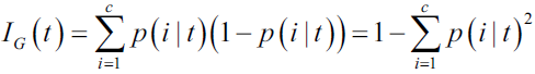OR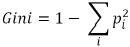
the split producing minimum Gini impurity will be selected as the split
), and expressed relative to the maximum.

A graphical representation of the variable importances in the Heart data is shown in Figure 8.9.We see the mean decrease in Gini index for each variable(features), relative to the largest. The variables with the largest mean decrease in Gini index are Thal, Ca, and ChestPain

###########

In other words, in building a random forest, at each split in the tree, the algorithm is not even allowed to consider a majority of the available predictors(the very best feature when splitting a node). This may sound crazy, but it has a clever rationale. Suppose that there is one very strong predictor in the data set, along with a number of other moderately strong predictors. Then in the collection of bagged trees, most or all of the trees will use this strong predictor in the top split. Consequently, all of the bagged trees will look quite similar to each other. Hence the predictions from the bagged trees will be highly correlated. Unfortunately, averaging many highly correlated quantities量 does not lead to as large of a reduction in variance as averaging many uncorrelated quantities.In particular, this means that bagging will not lead to a substantial reduction in variance over a single tree in this setting.

Random forests overcome this problem by forcing each split to consider only a subset of the predictors. Therefore, on average (p − m)/p of the splits will not even consider the strong predictor( p: the total p features in the traning set, m : the subset of p features ), and so other predictors will have more of a chance. We can think of this process as decorrelating去相关 the trees, thereby making the average of the resulting trees less variable and hence more reliable.

The main difference between bagging and random forests is the choice of predictor subset size m( m : the subset of p features ).

For instance, if a random forest is built using m = p, then this amounts simply to bagging其实等于建立装袋法树.

On the Heart data, random forests using $\large m = \sqrt{p}$ leads to a reduction in both test error:RandomForest
and OOB: RandomForest error over bagging (Figure 8.8).
( the training instances that are not sampled are called out-of-bag (oob) instances
The resulting OOB error is a valid estimate of the test error for the bagged model (bag_clf.oob_score_), since the response for each observation is predicted using only the trees that were not fit using that observation(likes each prediction was happened in their validation set)
OOB error is virtually equivalent to leave-one-out cross-validation error留一法交叉验证误差. The OOB approach for estimating the test error is particularly convenient when performing bagging on large data sets for which cross-validation would be computationally onerous麻烦的.
)
FIGURE 8.8. Bagging and random forest results for the Heart data. The test error (black and orange) is shown as a function of B, the number of different bootstrapped training sets used(n_estimators=B in sklearn). Random forests were applied with $\large m = \sqrt{p}$ . The dashed line indicates the test error resulting from a single classification tree. The green and blue traces show the OOB（out-of-bag） error, which in this case is considerably lower.

Extra-Trees or Extremely Randomized Trees

When you are growing a tree in a Random Forest, at each node only a random subset of the features is considered for splitting (as discussed earlier). It is possible to make trees even more random by also using random thresholds for each feature rather than searching for the best possible thresholds (like regular Decision Trees do).

A forest of such extremely random trees is simply called an Extremely Randomized Trees ensemble 极端随机树(or Extra-Trees for short). Once again, this trades more bias for a lower variance. It also makes Extra-Trees much faster to train than regular Random Forests since finding the best possible threshold for each feature at every node is one of the most time-consuming tasks of growing a tree.

You can create an Extra-Trees classifier using Scikit-Learn's ExtraTreesClassifier class. Its API is identical to the RandomForestClassifier class. Similarly, the Extra TreesRegressor class has the same API as the RandomForestRegressor class.
#############################
TIP
It is hard to tell in advance whether a RandomForestClassifier will perform better or worse than an ExtraTreesClassifier.
Generally, the only way to know is to try both and compare them using cross-validation (and tuning the hyperparameters using grid search).
#############################

In extremely randomized trees (see ExtraTreesClassifier and ExtraTreesRegressor classes), randomness goes one step further in the way splits are computed. As in random forests, a random subset of candidate features is used, but instead of looking for the most discriminative thresholds, thresholds are drawn at random for each candidate feature and the best of these randomly-generated thresholds is picked as the splitting rule. This usually allows to reduce the variance of the model a bit more, at the expense of a slightly greater increase in bias:

from sklearn.model_selection import cross_val_score
from sklearn.datasets import make_blobs
from sklearn.ensemble import RandomForestClassifier
from sklearn.ensemble import ExtraTreesClassifier
from sklearn.tree import DecisionTreeClassifier

X, y = make_blobs(n_samples=10000, n_features=10, centers=100,
                  random_state=0)

dt_clf = DecisionTreeClassifier(max_depth=None, min_samples_split=2,
                                max_features=None, # max_features=n_features.
                                random_state=0
                               )
dt_scores = cross_val_score(dt_clf, X, y, cv=5)
print( "dt_scores:" , dt_scores.mean() )

rf_clf = RandomForestClassifier(n_estimators=10, max_depth=None,
                                min_samples_split=2,
                                max_features='sqrt', ######
                                random_state=0)
rf_scores = cross_val_score(rf_clf, X, y, cv=5)
print( "rf_scores:" , rf_scores.mean() )

et_clf = ExtraTreesClassifier(n_estimators=10, max_depth=None,
                              min_samples_split=2,
                              max_features='sqrt', ######
                              random_state=0)
et_scores = cross_val_score(et_clf, X, y, cv=5)
print( "et_scores:" , et_scores.mean() )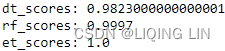

The sklearn.ensemble module provides a random forest regressor called RandomForestRegressor

More ensemble models

The sklearn.ensemble module contains various other ensemble regressors, as well as classifier models. More information can be found at https://scikit-learn.org/stable/modules/classes.html#module-sklearn.ensemble

Predicting trends with classification-based machine learning

Classification-based machine learning is a supervised machine learning approach in which a model learns from given input data and classifies it according to new observations. Classification may be

bi-class, such as identifying whether an option should be exercised or not,
or multi-class, such as the direction of a price change, which can be either up, down, or unchanging.

In this section, we will look again at creating cross-asset momentum models by having the prices of four diversified assets predict the daily trend of JPM on a daily basis for the year of 2018. The

prior 1-month and 3-month lagged returns of the S&P 500 stock index,
the 10-year treasury bond index, the US dollar index,
and gold prices

will be used to fit the model for prediction.

Our target variables consist of Boolean indicators, where

a True value indicates an increase or no-change from the previous trading day's closing price,
and a False value indicates a decrease.

Let's begin by preparing the dataset for our models.

Preparing the target variables

We have already downloaded the JPM dataset to the pandas DataFrame, df_jpm , in a previous section, and the y variable contains the daily percentage change of JPM. Convert these values to labels with the following code:

jpm_prices = yf.download( 'JPM' )['Adj Close']
y = jpm_prices.pct_change()
y

import numpy as np

# y.loc['2018']
y_direction = y>=0
y_direction

and

we can see that the y_direction variable becomes a pandas Series object of Boolean values. A percentage change of zero or more classifies the value with a True label, and False otherwise. Let's extract unique values with the unique() command as column names for use later on:

flags = list( y_direction.unique() )
flags.sort()
print(flags)

The column names are extracted to a variable called flags. With our target variables ready, let's continue to obtain our independent multi-asset variables.

Preparing the dataset of multiple assets as input variables

We will be reusing the pandas DataFrame variables, df_assets_1m and df_assets_3m, from the previous section containing the lagged 1-month and 3-month percentage returns of the 4 assets and combine them into a single variable, df_input , with the following code:

import yfinance as yf

# ^GSPC : SPX
# https://blog.csdn.net/Linli522362242/article/details/126269188
symbol_list = ['^GSPC','GLD','UUP','IEF']
symbols = ' '.join(symbol_list)

df = yf.download( symbols)
df_assets=df['Adj Close'].dropna()

# df_assets.columns : Index(['GLD', 'IEF', 'UUP', '^GSPC'], dtype='object')
# pct_change() : prices-prices.shift(1)/prices.shift(1)
# pct_change() : the percentage change over the prior period values
df_assets_1m = df_assets.pct_change( periods=21 )
df_assets_1m.columns = [ '%s_1m' % col 
                         for col in df_assets.columns
                       ]
df_assets_3m = df_assets.pct_change( periods=63 )
df_assets_3m.columns = [ '%s_3m' % col
                         for col in df_assets.columns
                       ]
df_assets_6m = df_assets.pct_change( periods=126 )
df_assets_6m.columns = [ '%s_6m' % col
                         for col in df_assets.columns
                       ]
df_assets_12m = df_assets.pct_change( periods=252 )
df_assets_12m.columns = [ '%s_12m' % col
                          for col in df_assets.columns
                        ]

df_lagged = df_assets_1m.join( df_assets_3m )\
                        .join( df_assets_6m )\
                        .join( df_assets_12m ).dropna()
df_lagged

df_input = df_assets_1m.join( df_assets_3m ).dropna()
df_input

Use the info() command to view its properties:

df_input.info()

The output is truncated, but you can see we have 8 features as our independent variables spanning the years 2007 to 2022. With our input and target variables created, let's explore the various classifiers available in scikit-learn for modeling.

y_direction = y_direction[ df_input.index[0].date() : ]
y_direction

Logistic regression

Despite its name, logistic regression is actually a linear model used for classification. It uses a logistic function, also known as a sigmoid function, to model the probabilities describing the possible outcomes of a single trial. A logistic function helps to map any real-valued number to a value between 0 and 1. A standard logistic function is written as follows:
OR

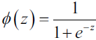
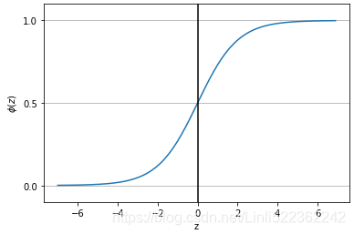
$\large e$ is the base of the natural logarithm, and
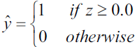
$\large x$ is the X-value of the sigmoid's midpoint.
$\large \hat{y}$ is the predicted real value between 0 and 1, to be converted to a binary equivalent of 0 or 1 either by rounding or a cut-off value.
==>==>
the logarithm of the odds ratio (log-odds):
==>

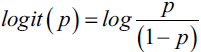
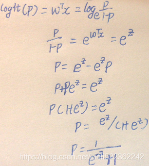is the conditional probability that a particular sample belongs to class 1 given the features of $\large x$ .
Minimize logistic cost function:
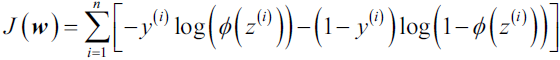
Minimize MSE: $\large J(w) = \frac{1}{n}\sum_{i=1}^{n} ( \phi(z^{(i)})-y^{(i)} )^2$ and $\large y^{(i)}$ is 0 or 1
  ==> $\large \frac{1}{1+e^{-w^T x}}$ OR $\large \frac{1}{1+e^{-\theta^T x}}$

==> $\large i$ is the index of current sample $\large x^i$
if $\large y$ =1 or $\large y^{(i)} = 1$ , Maximize  for closing to 1, and $\large ( 1-\phi(z^{(i)}) )^{ 1 - y^{(i)} }$ =1 ==>Maximize $\large ( \phi(z^{(i)}) )^{ 1 - y^{(i)} }$ to 1
if $\large y$ =0 or $\large y^{(i)} = 0$ , Minimize   for closing to 0, then $\large ( \phi(z^{(i)}) )^{ 1 - y^{(i)} }$ =1 ==>Maximize $\large ( 1-\phi(z^{(i)}) )^{ 1 - y^{(i)} }$ to 1
==>Convert to Maximize the likelihood, (y=0, 1)
==>Use logarithm to convert multiplication to addition:
==>Minimize log-likelihood:
the partial derivative of the log-likelihood function with respect to the jth weight:
Note: and

$\large \frac{\partial }{\partial w_j} l(w) = \left [ y \frac{1}{ \phi{(z)} } - (1-y) \frac{1}{1-\phi{(z)}} \right ] \frac{\partial }{\partial w_j} \phi(z)$ ### for each index $\large i$
Before we continue, let's also calculate the partial derivative of the sigmoid function: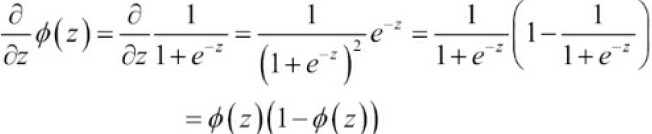

Note
Now, we can re-substitute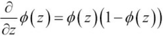 and in our first equation to obtain the following:
$\large j$ : the feature index in $\large x$

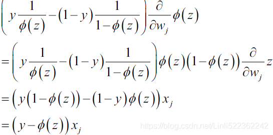
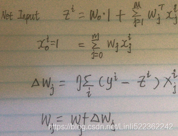
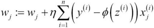m : the number of features for each $\large x^i$

class LogisticRegressionGD(object):
    """Logistic Regression Classifier using gradient descent.
    Parameters
    ------------
    eta : float
        Learning rate (between 0.0 and 1.0)
    n_iter : int
        Passes over the training dataset.
    random_state : int
        Random number generator seed for random weight
        initialization.
        
    Attributes
    -----------
    w_ : 1d-array
        Weights after fitting.
    cost_ : list
        Sum-of-squares cost function value in each epoch.
    """
    def __init__(self, eta=0.05, n_iter=100, random_state=1):
        self.eta = eta
        self.n_iter = n_iter
        self.random_state = random_state
    
    def net_input(self, X):
        #calculate net input
        return np.dot(X, self.w_[1:]) + self.w_[0] # z = w^T*X = w_0 + w_1*x_1 +... + w_m*x_m
    
    def activation(self, z):
        # compute logistic sigmoid activation
        # numpy.clip(a, a_min, a_max, out=None)
        return 1. / ( 1. + np.exp( -np.clip(z, -250, 250) ) )
        
    def fit(self, X, y):
        """ Fit training data.
        Parameters
        ----------
        X : {array-like}, shape = [n_samples, n_features]
            Training vectors, where n_samples is the number of
            samples and
            n_features is the number of features.
        y : array-like, shape = [n_samples]
            Target values.
        Returns
        -------
        self : object
        """
        
        rgen = np.random.RandomState(self.random_state)
                               # mean,  variance,       bias + number of features
        self.w_ = rgen.normal( loc=0.0, scale=0.01, size=1+X.shape[1])
        self.cost_ =[]
        
        for i in range(self.n_iter):
            net_input = self.net_input(X) # z = w^T*X = w_0 + w_1*x_1 +... + w_m*x_m
            output = self.activation(net_input) #logistic sigmoid function
            errors = (y-output)
            #Note: the weight update is calculated based on all samples in the training set 
            # X.T : (n_features, n_samples) #single column matrix
            self.w_[1:] += self.eta* X.T.dot(errors)
            self.w_[0] += self.eta*errors.sum() # self.eta* 1*errors.sum()
            
            # note that we compute the logistic 'cost' now
            # instead of the sum of errors cost
            cost = (-y.dot(np.log(output))
                    -( (1-y).dot(np.log(output)) )
                   )#note dot including a sum action
            self.cost_.append(cost)
            
        return self
    
    def predict(self, X):  
        #OR# np.where( self.activation( self.net_input(X) )>=0.5, 1,0 )
        return np.where( self.net_input(X)>=0.0, 1, 0)#return class label after unit step

cp3 sTourOfMLClassifiers_stratify_bincount_likelihood_logistic regression_odds ratio_decay_L2_sigmoi_LIQING LIN的博客-CSDN博客

The LogisticRegression class of the sklean.linear_model module implements logistic regression. Let's implement this classifier model by writing a new class named LogisticRegressionModel that extends LinearRegressionModel with the following code:

from sklearn.linear_model import LogisticRegression

class LogisticRegressionModel( LinearRegressionModel ):
    def get_model( self ):
        return LogisticRegression( solver='lbfgs' )

# Limited-memory BFGS : Limited memory quasi-Newton methods

# lbfgs：拟牛顿法的一种，利用损失函数二阶导数矩阵即海森矩阵来迭代优化损失函数http://www.seas.ucla.edu/~vandenbe/236C/lectures/qnewton.pdf

The same underlying linear regression logic is used in our new classifier model. The get_model() method is overridden to return an instance of the LogisticRegression classifier model, using the LBFGS solver algorithm in the optimization problem.

A paper on the limited-memory Broyden–Fletcher–Goldfarb–Shanno (LBFGS) algorithm for machine learning can be read at https://arxiv.org/pdf/1802.05374.pdf

Create an instance of this model and provide our data:

logistic_reg_model = LogisticRegressionModel()
logistic_reg_model.learn( df_input, y_direction, 
                          start_date='2008', end_date='2022',
                          lookback_period=100
                        )
logistic_reg_model.df_result

Since our target variables are Boolean values, the model outputs predict Boolean values as well. But how well does our model perform? In the following sections, we will explore risk metrics for measuring our predictions. These metrics are different from those used for regression-based predictions in earlier sections. Classification-based machine learning takes another approach for measuring output labels.

Risk metrics for measuring classification-based predictions

In this section, we will explore common risk metrics for measuring classification-based machine learning predictions, namely the confusion matrix, accuracy score, precision score, recall score, and F1 score.

Confusion matrix

A confusion matrix, or error matrix, is a square matrix that helps to visualize and describe the performance of a classification model for which the true values are known. The confusion_matrix function of the sklearn.metrics module helps to calculate this matrix for us, as shown in the following code:

from sklearn.metrics import confusion_matrix

df_result = logistic_reg_model.df_result    
actual = list(df_result['Actual']) # a vertical list
predicted = list(df_result['Predicted']) # a vertical list

matrix = confusion_matrix(actual, predicted)

matrix

print( "JPM percentage returns since 2018\n\n",
       pd.crosstab( np.array(actual), np.array(predicted),
                    rownames=['Actual'], colnames=['Predicted']
                  )
     )

We obtain the actual and predicted values as separate lists. Since we have two types of class labels, we obtain a two-by-two matrix. The heatmap module of the seaborn library helps us understand this matrix.

Seaborn is a data visualization library based on Matplotlib. It provides a high-level interface for drawing attractive and informative statistical graphics, and is a popular tool for data scientists. If you do not have Seaborn installed, simply run the command: pip install seaborn

Run the following Python codes to generate the confusion matrix:

%matplotlib inline
import seaborn as sns
import matplotlib.pyplot as plt

plt.subplots( figsize=(12,8) )
ax=sns.heatmap( matrix, 
             square=True, 
             annot=True, fmt='d', 
             cbar=True, # Whether to draw a colorbar.
             linecolor='white', linewidths = 1,
             xticklabels=True, yticklabels=True,
           )
plt.xlabel( 'Predicted' )
plt.ylabel( 'Actual', rotation=0 )

ax.xaxis.set_label_position('top')

ax.set_yticklabels(['$N$egative','$P$ositive'], rotation=0)
ax.xaxis.tick_top() # set the ticklabel position
# OR
#ax.tick_params(top=True, labeltop=True, bottom=False, labelbottom=False)
plt.title( 'JPM percentage returns since 2018\n', fontsize=12 )
plt.show()

%matplotlib inline
import seaborn as sns
import matplotlib.pyplot as plt

plt.subplots( figsize=(12,8) )
ax=sns.heatmap( matrix.T, 
             square=True, 
             annot=True, fmt='d', 
             cbar=False, 
             linecolor='white', linewidths = 1,
             xticklabels=flags, yticklabels=flags
           )
plt.xlabel( 'Actual' )
plt.ylabel( 'Predicted', rotation=0 )
ax.set_yticklabels(ax.get_yticklabels(), rotation=0)

plt.title( 'JPM percentage returns since 2018' )
plt.show()

Don't let the confusion matrix confuse you. Let's break down the numbers in a logical manner and see how easily a confusion matrix works. Starting from the left column, we have a total of 1819 samples(=731 + 1088) classified as False(actual),

of which the classifier predicted correctly 731 times, and these are known as true negatives (TNs).
However, the classifier predicted it wrongly 1088 times, and these are known as false negatives (FNs).

In the right column, we have a total of 1880 samples(=753 + 1127) belonging to the True class.

The classifier predicted wrongly 753 times, and these are known as false positives (FPs).
The classifier did predict correctly 1127 times though, and these are known as true positives (TPs).

These computed rates are used in other risk metrics, as we shall discover in the following sections.

Accuracy score

An accuracy score is the ratio of correct predictions to the total number of observations. By default, it is expressed as a fractional value between 0 and 1. When the accuracy score is 1.0, it means that the entire set of predicted labels in the sample matches with the true set of labels. The accuracy score can be written as follows: $\large \mathbf{accuracy( y, \hat{y} ) = \frac{1}{n} \sum_{i=0}^{n-1} I ( \hat{y}_i = y_i ) =\frac{ (TP+TN) }{ (TP+FP+FN+TN) }\textbf{}}$

Here, $I(x)$ is the indicator function that returns 1 for a correct prediction, and 0 otherwise. The accuracy_score function of the sklearn.metrics module calculates this score for us with the following code:

from sklearn.metrics import accuracy_score

print( 'accuracy_score:', 
       accuracy_score(actual, predicted)
     )

Accuracy = (TP+TN)/(TP+FP+FN+TN) = (1127+731) /(1127+753+1088+731) =1858/3699 = 0.5022979183563125

How many observations(samples, daily percentage returns) did we correctly label out of the entire set?

The accuracy score suggests that our model is correct 50% of the time. Accuracy scores are great at measuring symmetrical datasets where values of false positives and false negatives are almost the same. To evaluate the performance of our model fully, we need to look at other risk metrics.

Precision score

A precision score is the ratio of correctly predicted positive observations to the total number of predicted positive observations, and can be written as follows: $=\mathbf{\frac{TP}{TP+FP}}$

This gives a precision score between 0 and 1, with 1 as the best value indicating that the model classifies correctly all the time. The precision_score function of the sklearn. metrics module calculates this score for us with the following code:

from sklearn.metrics import precision_score

print( 'Precision_Score:',
       precision_score( actual, predicted )
     )

How many of those daily percentage returns that we labeled as positive returns are actually positive returns?

The precision score suggests that our model is able to predict a classification correctly 51% of the time.

classification_report

from sklearn.metrics import classification_report

print( 'classification_report:\n',
       classification_report(actual,predicted)
     )

macro avg: 进行简单算术平均 unweighted mean; AllClassesAreEquallyImportant
0.50 = (0.49+0.51)/2 ... 0.50= (0.44+0.55)/2 # 2 classes or 2 labels
Note: 2 since there exist 2 possible values(0,1)

weighted avg: (start from left bottom)
0.50=(0.44*1819+0.55*1880)/(1819+1880) : 1819 and1880 are weights or supports
https://blog.csdn.net/Linli522362242/article/details/126502997

https://blog.csdn.net/Linli522362242/article/details/109560084

The scoring metrics that we've discussed so far are specific to binary classification systems. However, scikit-learn also implements macro and micro averaging methods
to extend those scoring metrics to multiclass problems via one-vs.-all (OvA) classification. The micro-average is calculated from the individual TPs, TNs, FPs, and FNs of the system. For example, the micro-average of the precision score in a k-class system can be calculated as follows:

The macro-average is simply calculated as the average scores of the different systems:

Micro-averaging is useful if we want to weight each instance or prediction equally, whereas macro-averaging weights all classes equally to evaluate the overall performance of a classifier with regard to the most frequent class labels.

If we are using binary performance metrics to evaluate multiclass classification models in scikit-learn, a normalized or weighted variant of the macro-average is used by default. The weighted macro-average is calculated by weighting the score of each class label by the number of true instances when calculating the average. The weighted macro-average is useful if we are dealing with class imbalances, that is, different numbers of instances for each label.

Recall score (aka Sensitivity)

The recall score is the ratio of correctly predicted positive observations to all the positive observations in the actual class, and can be written as follows:
$\mathbf{=\frac{TP}{TP+FN}}$

This gives a recall score of between 0 and 1, with 1 as the best value. The recall_score function of the sklearn. metrics module calculates this score for us with the following code:

from sklearn.metrics import recall_score

print( 'Recall_Score:', recall_score( actual, predicted) )

<==

Of all the people who are daily positive returns (target), how many of those we correctly predict?

The recall score suggests that our logistic regression model correctly identifies positive samples 60% of the time.

F1 score (aka F-Score or F-Measure)

The F1 score, or F-measure, is the weighted average of the precision score and the recall score, and can be written as follows:

This gives an F1 score between 0 and 1. When either the precision score or the recall score is 0, the F1 score will be 0. However, when both the precision score and recall score are positive, the F1 score gives equal weights to both measures. Maximizing the F1 score creates a balanced classification model with optimal balance of recall and precision. Oppositely F1 Score isn’t so high if one measure is improved at the expense of the other 相反，如果以牺牲另一项为代价来改进一项措施，那么 F1 分数就不会那么高.

from sklearn.metrics import f1_score

print( 'f1_score:', f1_score( actual, predicted) )

<==

The F1 score of our logistic regression model is 0.55.

Support vector classifier

A support vector classifier (SVC) is a concept of a support vector machine (SVM) that uses support vectors for classifying datasets.

More information on SVMs can be found at http: //www.statsoft.com/textbook/support-vector-machines.OR cp3 ML Classifiers_2_support vector_Maximum margin_soft margin_C~slack_kernel_Gini_pydot+_Infor Gai_LIQING LIN的博客-CSDN博客 OR https://www.sciencedirect.com/topics/mathematics/support-vector-machine OR https://blog.csdn.net/Linli522362242/article/details/104151351

Distance from point Q=(x1,y1,z1) to plane Ax+By+Cz+D=0 the distance d of a point Q=(x1,y1,z1) to a plane is determined by normal vector(法向量) $\vec{n}$ OR N=(A,B,C) and point P=(x0,y0,z0). The equation for the plane determined by N and P is A(x−x0)+B(y−y0)+C(z−z0)=0, which we could write as Ax+By+Cz+D=0, where D=−Ax0−By0−Cz=0. (Ax+By+Cz −A*x0−B*y0−C*z0=0)
a unit normal vector N:

the distance d >=0 from Q to the plane, is simply the length of the projection of vector PQ onto the unit normal vector N or $\vec{n}$ .

note: the dot product（内积） and $\vec{PQ} = (x_1 - x_0, y_1 - y_0, z_1 - z_0)$

==>

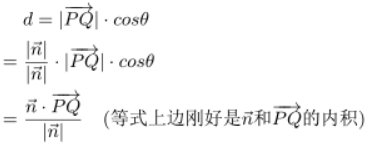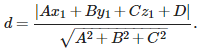
the planeAx+By+Cz+D=0 is a separating hyperplane(N=(A,B,C) is vector W, b=D=−Ax0−By0−Cz0=0 , point P=(x0,y0,z0) is in this hyperplane) in Support Vector Machines, and it has another form =0 OR =0

the formula of the distance for any data point to the separating hyperplane is $\frac{W^TA + b}{\left \| b \right \|} = \frac{W^T X + b}{\left \| b \right \|} \geq 1$ (constraints) note A = X (X is a vector, a data point with some features, x0, x1 ... Xn, the following example just use two features)

Here, N is the number of samples in our dataset.

Positive hyperplane :
Negative hyperplane:
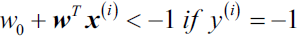
==>(constraint) and $w_0 = b$

The goal now is to find the w and b values that will define our classifier. To do this, we must find the points with the smallest margin (the shortest perpendicular distance between the decision boundary(separating hyperplane) and the closest of data points). (Some of these data points are selected as the support vectors to maximize that margin). Then, when we find the points with the smallest margin, we must maximize that margin .
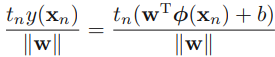OR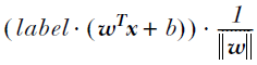

the distance of a point to the decision surface/boundary is given by

The margin is given by the perpendicular distance to the closest data point from the data set,
and we wish to optimize the parameters w and b in order to maximize this distance(maximizing the margin leads to a particular choice of decision boundary, the location of this boundary is determined by a subset of the datapoints, known as support vectors). Thus the maximum margin solution is found by solving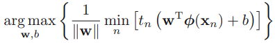

sub-Summary: to solve
==>At first,(to find the closest of data points to decision boundary),
Then maximize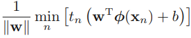 for maximizing the margin( to choose the decision boundary or to find the support vectors that determine the location boundary) ==> (maximize ==> is equivalent to minimizing )
==>

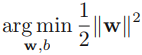
In order to solve this constrained optimization (maximize) problem, we introduce Lagrange multipliers拉格朗日乘数 $a_n \geq 0$ , with one multiplier $a_n$ for each of the constraints in (7.5==>), giving the Lagrangian function ###we put the constraints together
where a = . Note the minus sign in front of the Lagrange multiplier term, because we are minimizing with respect to w and b, and maximizing with respect to $\large \max_{a_n\geq 0} L(W,b,a)$ OR $\large \max_{a_i\geq 0} L(W,b,a)$ for .
==>convert to==>
Setting the derivatives of L(w, b, a) with respect to w and b equal to zero, we obtain the following two conditions

the partial derivatives of L (w, b, a)=0 ==>==>
the partial derivatives of L (w, b, a)=0 ==>==>

Eliminating w and b from L(w, b, a) using these conditions

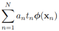replaced with $\mathbf{\frac{1}{2} \left \| W \right \|^2} = \mathbf{ \frac{1}{2} W^T W } =$ *

and,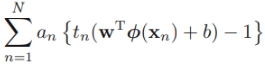
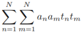
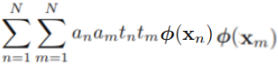== $\sum_{n=1}^{N}a_n t_n b -\sum_{n=1}^{N} a_n$
==> +0 $-\sum_{n=1}^{N} a_n$

Then,

minus==>==>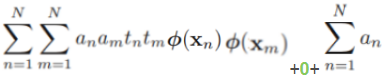

==>

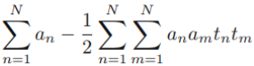
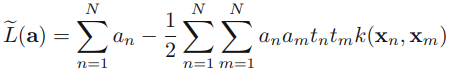
then gives the dual representation of the maximum margin problem in which we maximize
with respect to a subject to the constraints

With the introduction of something called slack variables, we can allow some data points to be on the wrong side of the decision boundary. Our optimization goal stays the same, but we now have a new set of constraints:
The constant C controls weighting between our goal of making the margin large and ensuring that most of the data points have a functional margin of at least 1.0. The majority of the work in SVMs is finding the alphas.
with ξn > 1 will be misclassified. The exact classification constraints (7.5: <==) are then replaced with Points for which lie inside the margin, but on the correct side of the decision boundary
Our goal is now to maximize the margin while softly penalizing points that lie on the wrong side of the margin boundary. We therefore minimize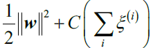

We now wish to minimize (7.21) subject to the constraints (7.20) together with. The corresponding Lagrangian is given by

where { 0} and { 0} are Lagrange multipliers. The corresponding set of KKT conditions are given by
where n = 1,...,N.
We now optimize out w, b, and {ξn} making use of the definition (7.1 ) of y(x) to give

Using these results to eliminate w, b, and {ξn} from the Lagrangian, we obtain the dual Lagrangian in the form

which is identical to the separable case(7.10), except that the constraints are somewhat different. To see what these constraints are, we note that is required because these are Lagrange multipliers. Furthermore, (7.31) together with implies an C. We therefore have to minimize (7.32) with respect to the dual variables { $\large a_n$ } subject tofor n = 1,...,N, where (7.33) are known as box constraints. This again represents a quadratic programming problem. If we substitute (7.29) into (7.1), we see that predictions for new data points are again made by using (7.13).

We can now interpret the resulting solution. As before,

a subset of the data points may have $\large a_n = 0$ , in which case they do not contribute to the predictive model (7.13). The remaining data points constitute the support vectors.
These have $\large a_n > 0$ and hence from (7.25) must satisfy
If $\large a_n < C$ , then (7.31) implies that $\large \mu_n > 0$ , which from (7.28) requires ξn = 0 and hence such points lie on the margin.
Points with $\large a_n = C$ can lie inside the margin and can either be correctly classified if $\large \xi_n \leqslant 1$ or misclassified if ξn > 1.

The SVC class of the sklean.svm module implements the SVM classifier. Write a class named SVCModel and extend LogisticRegressionModel with the following code:

The parameter C is therefore analogous相似的 to (the inverse of) a regularization coefficient正则化的强度与C成反比 because it controls the trade-off between minimizing training errors and controlling model complexity. In the limit C → ∞, we will recover the earlier support vector machine for separable data.

VS05_Support Vector Machines_02_Polynomial Kernel_Gaussian RBF_Kernelized SVM Regression_Quadratic Pro_LIQING LIN的博客-CSDN博客

from sklearn.svm import SVC

class SVCModel( LogisticRegressionModel ):
    def get_model( self ):
        # default kernel='rbf'
        # gamma='auto', uses 1/n_features
        return SVC(C=1000, gamma='auto')

svc_model = SVCModel()
svc_model.learn( df_input, y_direction,
                 start_date='2018', end_date='2022',
                 lookback_period=100
               )

Here, we are overriding the get_model() method to return the SVC class of scikit-learn. A high-penalty C value of 1000 is specified. The gamma parameter is the kernel coefficient with a default value of auto . The learn() command is executed with our usual model parameters. With that, let's run the risk metrics on this model:

df_result = svc_model.df_result
actual = list( df_result['Actual'] )
predicted = list( df_result['Predicted'] )

print( 'accuracy_score:', accuracy_score(actual, predicted) )
print( 'precision_score:', precision_score(actual, predicted) )
print( 'recall_score:', recall_score(actual, predicted) )
print( 'f1_score:', f1_score(actual, predicted) )

We obtain better scores(accuracy score and precision_score) than from the logistic regression classifier model. By default, the C value of the linear SVM is 1.0, which would in practice give us generally comparable performance with the logistic regression model. There is absolutely no rule of thumb for choosing a C value, as it depends entirely on the training dataset. A nonlinear SVM kernel can be considered by supplying a kernel parameter to the SVC() model. More information on SVM kernels is available at https: //scikit-learn.org/stable/modules/svm.html#svm-kernels

Stochastic gradient descent

04_TrainingModels_Normal Equation(正态方程,正规方程) Derivation_Gradient Descent_Polynomial Regression_LIQING LIN的博客-CSDN博客

Stochastic gradient descent (SGD) is a form of gradient descent that works by using an iterative process to estimate the gradient towards minimizing an objective loss function, such as a linear support vector machine or logistic regression. The stochastic term comes about as samples are chosen at random. When lesser iterations are used, bigger steps are taken to reach the solution, and the model is said to have a high learning rate. Likewise, with more iterations, smaller steps are taken, resulting in a model with a small learning rate. SGD is a popular choice of machine learning algorithm among practitioners as it has been effectively used in large-scale text classification and natural language processing models.

The SGDClassifier class of the sklearn.linear_model module implements the SGD classifier.

Linear discriminant analysis

Linear discriminant analysis (LDA) is a classic classifier that uses a linear decision surface, where the mean and variance for every class of the data is estimated. It assumes that the data is Gaussian(One assumption in LDA is that the data is normally distributed), and that each attribute has the same variance(the features are statistically independent of each other), and values of each variable are around the mean. LDA computes discriminant scores by using Bayes' theorem for each observation to determine to which class it belongs.

The LinearDiscriminantAnalysis class of the sklearn.discriminant_analysis module implements the LDA classifier. cp5_Compressing Data via Dimensionality Reduction_feature extraction_PCA_LDA_convergence_kernel PCA_LIQING LIN的博客-CSDN博客

Quadratic discriminant analysis

Quadratic discriminant analysis (QDA) is very similar to LDA, but uses a quadratic decision boundary and each class uses its own estimate of variance. Running the risk metrics shows that the QDA model does not necessarily give better performance than the LDA model. The type of decision boundary has to be taken into consideration for the model required. QDA is better suited for large datasets, as it tends to have a lower bias and higher variance. On the other hand, LDA is suitable for smaller datasets that have a lower bias and a higher variance.

The QuadraticDiscriminantAnalysis class of the sklearn.discriminant_analysis module implements the QDA model.

KNN classifier

The k-nearest neighbors (k-NN) classifier is a simple algorithm that conducts a simple majority vote of the nearest neighbors of each point, and that point is assigned to a class that has the most representatives within the nearest neighbors of the point. While there is not a need to train a model for generalization, the predicting phase is slower and costlier in terms of time and memory.mpf9_Backtesting_mean-reverting_threshold_model_Survivorship bias_sklearn打印默认参数_Gini_k-mean_knn_CART_LIQING LIN的博客-CSDN博客

The KNeighborsClassifier class of the sklearn.neighbors module implements the KNN classifier.

Conclusion on the use of machine learning algorithms

You may have observed that predicted values from our models are far off from actual values. This chapter aims to demonstrate the best of the machine learning features that scikit-learn offers, which may possibly be used to predict time series data. No studies to date have shown that machine learning algorithms can predict prices even close to 100% of the time. A lot more effort goes into building and running machine learning systems effectively.

Summary

In this chapter, we have been introduced to machine learning in the context of finance. We discussed how AI and machine learning is transforming the financial sector. Machine learning can be supervised or unsupervised, and supervised algorithms can be regression- based and classification-based. The scikit-learn Python library provides various machine learning algorithms and risk metrics.

We discussed the use of regression-based machine learning models such as OLS regression, ridge regression, LASSO regression, and elastic net regularization in predicting continuous values such as security prices. An ensemble of decision trees was also discussed, such as the bagging regressor, gradient tree boosting, and random forests. To measure the performance of regression models, we visited the MSE, MAE, explained variance score, and R2 score.

Classification-based machine learning classifies input values as classes or labels. Such classes may be bi-class or multi-class. We discussed the use of logistic regression, SVC, LDA and QDA, and k-NN classifiers for predicting price trends. To measure the performance of classification models, we visited the confusion matrix, accuracy score, precision and recall scores, as well as the F1 score.

In the next chapter, we will explore the use of deep learning in finance.

LIQING LIN

关注

2
点赞
踩
0

收藏

觉得还不错? 一键收藏
0
评论
mpf10_yfinan_Explained variance_R2_ols_cointegration_Gradient Boost_lbfgs_热力图sns ticklabel_SVM_confu

mpf10_yfinan_Explained variance_cointegration_Gradient Boost_lbfgs_sns ticklabel_SVM svc_confusion matrix_heatmap_accuracy score, precision score, recall score, F1 score_MSE, MAE, explained variance score, R2 score_OLS, ridge, LASSO, elastic net, L1 L2正则
复制链接

扫一扫