Brief
About 3D point cloud up-sampling from Xianzhi Li’s work:
Detail
Backgroud
Due to the sparseness and irregularity of the point cloud, learning a deep net on point cloud remains a challenging work. Recent work have been trying to accomplish upsampling based on some prior knowledge and assumption, also some external input and information such as normal vector. What’s more, some works trying to extract features directly from the point cloud are always running into problem of missing semantic information and getting a different shape of point cloud from the original one. Since semantic information can be captured through deep net, it came to authors’ mind that maybe they could bring about a break-through in point upsampling by using the deep net to extract features from target point cloud.
PU-Net
Challenges in learning features from point cloud with deep net:
- How to prepared enough training dataset
- How to expand the number of points
- How to design loss function
Dataset Preparation
Due to there are only mesh data available, they then decide to create their training data from the those data:
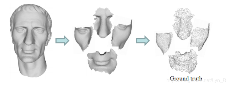
- As upsampling can be treated as a work on local region of a image, firstly they splits the mesh data into several separated parts, regrading each of which as a patch
- Then, they transform mesh surface into dense point cloud through poisson disk sampling. By this they can obtain their ground truth
- Last is to produce input from the ground truth. Since there are more than exacly one input corresponding, on-the-fly inputs are generated by randomly sampled from the ground truth point sets with a fixed downsampling rate r.

Figure.1 from mesh to densy point cloud as ground truth
With 40 mesh splitted into 1000 patches, a 4k-size training dataset is now available, with each patch consists of input and corresponding ground truth.
Expansion of Points in Point Cloud
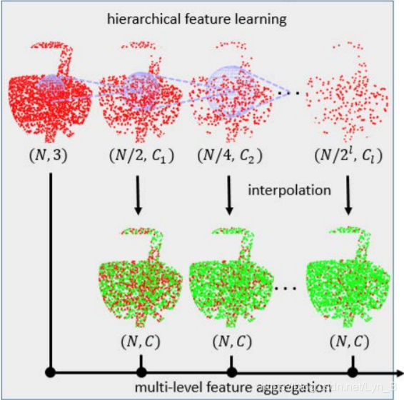
First of all, we need to extract features from the local region in the point cloud, required to perform the extraction on each point in the cloud since local features is expected for solution of upsampling problem. They construct a network similar to PointNet++. As shown in the following figure, we can see that features are extracted from different levels of resolution of the point clouds generated by a exponential downsampling starting from the original one. In each layer, green points are generated by interpolation from nearest red points. Only the output of the last layer is accepted in PointNet++. However, as we have been mentioning above, local feature is required in upsampling problem, so in PU-Net they concat each feature map attained from each layer to produce the final output of this hierarchical feature learning network.

Figure.2 PU-Net hierarchical feature learning which is more helpful for upsampling task
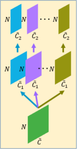
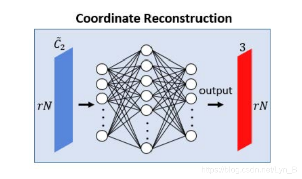
The expansion is carried out in feature space. That means they do not directly expand points in the point cloud according to the features extracted, instead they expand feature map using different convolutional kernel in feature space, reshape and finally regress the 3D coordinates by a fully connected layer. The expansion is shown in the following picture:

Figure.3 Expansion in feature space from NxC to NxrC
The expansion operation can be represented as the following function:
f
′
=
R
S
(
[
C
1
2
(
C
1
1
(
f
)
)
,
…
,
C
r
2
(
C
r
1
(
f
)
)
]
)
f'=\mathcal{RS([C_{1}^{2}(C_{1}^{1}(f)),\dots,C_{r}^{2}(C_{r}^{1}(f))])}
f′=RS([C12(C11(f)),…,Cr2(Cr1(f))])
in which:
- R S \mathcal{RS} RS is the reshape function
- C r 2 , C r 1 \mathcal{C_{r}^{2},C_{r}^{1}} Cr2,Cr1 represent the second time and first time convolution with kernel r alternatively

Note that two times of convolution is performed in order to break points’ correlation, 'cause points generated from the same feature map, although different convolutional kernel is applied, usually gather togather. It’s much better to use different convolutional kernel to perform a two-time convolution to ensure a much more uniform generation.
Construction of Loss Function
Two basic requirement:
- points generated should be uniform
- points generated should be informative and should not cluster
Two loss functions are designed to ensure satisfactory points’ distribution listed above.
The First one is call reconstruction loss using an Earth Movers Distance, namely EMD, which is famous for evaluating least distance to transform one distribution to another. By means of this evaluation, points generated will be engaged to be on the surface and outliers will be punished, gradually moving towards the surface through iterations. The loss function can be represented as follow:
L
r
e
c
=
d
E
M
D
(
S
p
,
s
g
t
)
=
min
Ø
:
S
p
→
S
g
t
∑
x
i
∈
S
p
∣
∣
x
i
−
Ø
(
x
i
)
∣
∣
2
L_{rec}=d_{EMD}(S_{p},s_{gt})=\min_{\text\O:S_{p}\rightarrow S_{gt}}\sum_{x_{i}\in S_{p}}||x_{i}-\text\O(x_{i})||_{2}
Lrec=dEMD(Sp,sgt)=Ø:Sp→Sgtminxi∈Sp∑∣∣xi−Ø(xi)∣∣2
with:
- S p S_{p} Sp is the predicted point and S g t S_{gt} Sgt is the ground truth
- Ø : S p → S g t \text\O:S_{p}\rightarrow S_{gt} Ø:Sp→Sgt inddicates the bijection mapping
The second one is call repulsion loss which will punish those points clustering to ensure a much more uniform distribution. The loss function can be represented as follow:
L
r
e
p
=
∑
i
=
0
N
^
∑
i
′
∈
K
(
i
)
η
(
∣
∣
x
i
′
−
x
i
∣
∣
)
w
(
∣
∣
x
i
′
−
x
i
∣
∣
)
L_{rep}=\sum_{i=0}^{\hat{N}}\sum_{i'\in K(i)}\eta(||x_{i'}-x_{i}||)w(||x_{i'}-x_{i}||)
Lrep=i=0∑N^i′∈K(i)∑η(∣∣xi′−xi∣∣)w(∣∣xi′−xi∣∣)
with:
- N ^ \hat N N^ is the number of output points
- K ( i ) K(i) K(i) are the k nearest point of x_{i}
- repulsion term: η ( r ) = − r \eta(r)=-r η(r)=−r
- fast-decaying weight function: w ( r ) = e − r 2 / h 2 w(r)=e^{-r^{2}/h^{2}} w(r)=e−r2/h2, which will decrease over downsampling
Contribution
Their work is first to apply deep net in point cloud upsampling, which can capture much more features in the point cloud and present us a better solution compared with those traditional solution which directly extract features from point cloud.
Consideration
As Xinzhi Li showed in GAMES Webinar 120, she told us that PU-Net, although having performed well in upsampling point cloud generation, doesn’t have the capability of edge detection resulting in a tough surface on some regular object like legs of a chair. That’s why they came up with a new work in the same year called EC-Net, namely Edge-aware Point set Consolidation Network, which was accepted in ECCV 2018.


 852
852

 被折叠的 条评论
为什么被折叠?


