


文章目录
图片增强
为什么要使用图片增强
数据增强是一种常用的神经网络优化技术,旨在加速神经网络的训练并提高其性能1. 数据增强的作用是让有限的数据产生更多的数据,增加训练样本的数量以及多样性(噪声数据),提升模型鲁棒性,或者你可以进行理解,数据增强后就是将原本图片的主体进行平移,当然不仅只有平移,放大缩小,然后需求我们的模型仍然可以识别出这个图片。
详细的参数介绍:链接
具体方式
参数可见上面的帖子,上面有进行详细的介绍:
import tensorflow as tf
from PIL import Image
import matplotlib.pyplot as plt
import numpy as np
# from tensorflow.keras.preprocessing.image import ImageDataGenerator
# from tensorflow.keras.datasets import cifar10

img = Image.open("./mm.jpg")
plt.imshow(img)
plt.axis("off")
plt.show()

img_array = np.array(img, dtype=np.float32)
img_array = np.expand_dims(img_array, axis=0)
print(img_array.shape)
输出:
图片见下
(1, 1080, 1080, 3)

datagen = tf.keras.preprocessing.image.ImageDataGenerator(
    rotation_range=90,  # 旋转
#     shear_range=0.5,  # 剪切角度
#     shear_range=20.0,
#     horizontal_flip=True  # 水平翻转
#     vertical_flip=True,  # 垂直翻转
)

datagen.fit(img_array)
my_generator = datagen.flow(img_array, batch_size=1)
res = my_generator.next()
print(res.shape)

plt.imshow(np.int_(res[0]))
plt.axis("off")
plt.show()
输出:
(1, 1080, 1080, 3)
图片见下

datagen = tf.keras.preprocessing.image.ImageDataGenerator(
#     rotation_range=20,
    shear_range=50.0,
#     horizontal_flip=True  # 水平翻转
#     vertical_flip=True,  # 垂直翻转
)

datagen.fit(img_array)
my_generator = datagen.flow(img_array, batch_size=1)
res = my_generator.next()
print(res.shape)

plt.imshow(np.int_(res[0]))
plt.axis("off")
plt.show()
输出:
(1, 1080, 1080, 3)
图片见下

.flow_from_directory(directory)
这个适用于一个标签一个文件夹的情况
train_datagen = ImageDataGenerator(
        rescale=1./255,
        shear_range=0.2,
        zoom_range=0.2,
        horizontal_flip=True)
test_datagen = ImageDataGenerator(rescale=1./255)
train_generator = train_datagen.flow_from_directory(
        'data/train',
        target_size=(150, 150),
        batch_size=32,
        class_mode='binary')
validation_generator = test_datagen.flow_from_directory(
        'data/validation',
        target_size=(150, 150),
        batch_size=32,
        class_mode='binary')
model.fit(
        train_generator,
        steps_per_epoch=2000,
        epochs=50,
        validation_data=validation_generator,
        validation_steps=800)
例子可见下面的resnet50的fine-tune
flow_from_dataframe
这个适用于需要自己去调整标签的情况
flow_from_dataframe(
    dataframe,
    directory=None,
    x_col='filename',
    y_col='class',
    weight_col=None,
    target_size=(256, 256),
    color_mode='rgb',
    classes=None,
    class_mode='categorical',
    batch_size=32,
    shuffle=True,
    seed=None,
    save_to_dir=None,
    save_prefix='',
    save_format='png',
    subset=None,
    interpolation='nearest',
    validate_filenames=True,
    **kwargs
)
例子:
train_lables_file = '../cifar10/trainLabels.csv'
def parse_csv_file(filepath, folder):
    """Parses csv files into (filename(path), label) format"""
    results = []
    #读取所有行
    with open(filepath, 'r') as f:
#         lines = f.readlines()  为什么加[1:],可以试这个
        lines = f.readlines()[1:]
    for line in lines:
        image_id, label_str = line.strip('\n').split(',')
        image_full_path = os.path.join(folder, image_id + '.png')
        results.append((image_full_path, label_str))
    return results
train_labels_info = parse_csv_file(train_lables_file, train_folder)
train_df = pd.DataFrame(train_labels_info[0:45000])
train_df.columns = ['filepath', 'class']
train_datagen = keras.preprocessing.image.ImageDataGenerator(
    rescale = 1./255,
    rotation_range = 40,
    width_shift_range = 0.2,
    height_shift_range = 0.2,
    shear_range = 0.2,
    zoom_range = 0.2,
    horizontal_flip = True,
    fill_mode = 'nearest',
)
train_generator = train_datagen.flow_from_dataframe(
    train_df,
    directory = './',
    x_col = 'filepath',
    y_col = 'class',
    #讲labels转换为id
    classes = class_names,
    target_size = (height, width),
    batch_size = batch_size,
    seed = 7,
    shuffle = True,
    class_mode = 'sparse',
)
迁移学习(Transfer Learning)
迁移学习是什么意思呢?类比到我们人身上就是:我们可以这么理解就是拿学别的内容产生的知识,去做知识迁移,然后再学点一些新的知识,来做到相关的效果。
具体到模型身上就是,我们拿大佬已经训练好的相关的网络进行再次训练,加上我们自己的知识进行迁移,然后得到更好的效果,也称作fine-tune。
相关补充:链接
AlexNet

在AlexNet当中首次引入了relu 这种非线性的激活函数,然后可以发现,使用这种非线性的激活函数可以让目标函数更快收敛。
然后就是在全连接层当中加上了dropout,在AlexNet中设置的失活概率为0.5,在测试的时候,再使用所用的神经元但是要给它们的输出都乘以0.5。
更多补充:链接
VGG
在VGG当中更多的使用33,替代了AlexNet当中使用的1111 以及77,原因就是视野域,2层33的卷积实际上就等效于一层55的卷积,但是参数却比55来的小,并且还多一层激活函数,这样子的效果是非常好的。
resnet50
深层次网络训练瓶颈:梯度消失,网络退化
深度卷积网络自然的整合了低中高不同层次的特征,特征的层次可以靠加深网络的层次来丰富。从而,在构建卷积网络时,网络的深度越高,可抽取的特征层次就越丰富。所以一般我们会倾向于使用更深层次的网络结构,以便取得更高层次的特征。但是在使用深层次的网络结构时我们会遇到两个问题,梯度消失,梯度爆炸问题和网络退化的问题。
但是当使用更深层的网络时,会发生梯度消失、爆炸问题,这个问题很大程度通过标准的初始化和正则化层来基本解决,这样可以确保几十层的网络能够收敛,但是随着网络层数的增加,梯度消失或者爆炸的问题仍然存在。
还有一个问题就是网络的退化,举个例子,假设已经有了一个最优化的网络结构,是18层。当我们设计网络结构的时候,我们并不知道具体多少层次的网络时最优化的网络结构,假设设计了34层网络结构。那么多出来的16层其实是冗余的,我们希望训练网络的过程中,模型能够自己训练这五层为恒等映射,也就是经过这层时的输入与输出完全一样。但是往往模型很难将这16层恒等映射的参数学习正确,那么就一定会不比最优化的18层网络结构性能好,这就是随着网络深度增加,模型会产生退化现象。它不是由过拟合产生的,而是由冗余的网络层学习了不是恒等映射的参数造成的.
也就是说,由于我们多创建了多层网络,但是机器很难自己学到是把那些多余的层数学习成毫不影响,直接做到多余的层数我们输入x输出还是x,但是事实证明难以学到这种效果,但是机器容易学到0,也就是有了次个模型诞生的意义。
利用残差来替代之前的传入:
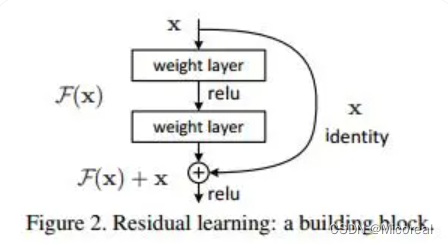
我们发现,假设该层是冗余的,在引入ResNet之前,我们想让该层学习到的参数能够满足h(x)=x,即输入是x,经过该冗余层后,输出仍然为x。但是可以看见,要想学习h(x)=x恒等映射时的这层参数时比较困难的。ResNet想到避免去学习该层恒等映射的参数,使用了如上图的结构,让h(x)=F(x)+x;这里的F(x)我们称作残差项,我们发现,要想让该冗余层能够恒等映射,我们只需要学习F(x)=0。学习F(x)=0比学习h(x)=x要简单,因为一般每层网络中的参数初始化偏向于0,这样在相比于更新该网络层的参数来学习h(x)=x,该冗余层学习F(x)=0的更新参数能够更快收敛。
代码学习
需要注意的是resnet50 他的输入图片是固定好的,应该是(None,224,224,3),所以一开始就需要进行相关的调整图片的大小。
import matplotlib as mpl
import matplotlib.pyplot as plt
%matplotlib inline
import numpy as np
import os
import pandas as pd
import sklearn
import sys
import tensorflow as tf
import time
from tensorflow import keras

# 处理数据
# -----------------------------------------------------------------------------
train_dir = "./datasets/10-monkey-species/training/training"
valid_dir = "./datasets/10-monkey-species/validation/validation"
label_file = "./datasets/10-monkey-species/monkey_labels.txt"
labels = pd.read_csv(label_file, header=0)
# 下面是resnet50规定的输入图片的尺寸大小
height = 224
width = 224
channels = 3
batch_size = 24
num_classes = 10
# 数据增强
# preprocessing_function这个参数是一个接受一个图像数组并返回一个处理后的图像数组的函数,用于在图像预处理时对每个输入的图像应用一个自定义的函数。
# 在这里,您使用了keras.applications.resnet50.preprocess_input作为这个参数的值,
# 这个函数是专门为resnet50模型设计的图像预处理函数,它会对图像进行归一化、中心化、裁剪等操作,以适应resnet50模型的输入要求。
# rotation_range:这个参数是一个整数,表示数据增强时图片随机旋转的角度范围。
# 在这里,您设置了rotation_range为40,表示每个图像在训练时会随机旋转0到40度之间的任意角度。
# width_shift_range:这个参数是一个浮点数,表示数据增强时图片水平平移的比例范围。
# 在这里,您设置了width_shift_range为0.2,表示每个图像在训练时会随机水平平移宽度的0到0.2倍之间的任意距离。
# height_shift_range:这个参数是一个浮点数,表示数据增强时图片垂直平移的比例范围。
# 在这里,您设置了height_shift_range为0.2,表示每个图像在训练时会随机垂直平移高度的0到0.2倍之间的任意距离。
# shear_range:这个参数是一个浮点数,表示数据增强时图片剪切变换的角度范围。
# 在这里,您设置了shear_range为0.2,表示每个图像在训练时会随机剪切变换0到0.2弧度之间的任意角度2。
# zoom_range:这个参数是一个浮点数或者一个列表,表示数据增强时图片缩放的比例范围。
# 在这里,您设置了zoom_range为0.2,表示每个图像在训练时会随机缩放0.8到1.2倍之间的任意比例2。
# horizontal_flip:这个参数是一个布尔值,表示数据增强时是否进行随机水平翻转。
# 在这里,您设置了horizontal_flip为True,表示每个图像在训练时有一半的概率会被水平翻转2。
# fill_mode:这个参数是一个字符串,表示当进行变换时超出边界的点如何处理。
# 在这里,您设置了fill_mode为’nearest’,表示超出边界的点会用最近邻的点填充2。
train_datagen = keras.preprocessing.image.ImageDataGenerator(
    preprocessing_function = keras.applications.resnet50.preprocess_input,
    rotation_range = 40,
    width_shift_range = 0.2,
    height_shift_range = 0.2,
    shear_range = 0.2,
    zoom_range = 0.2,
    horizontal_flip = True,
    fill_mode = 'nearest',
)
# 这里也需要修改 验证集只需要做那个缩放到224,224,3即可 其他的数据增强不需要搞
valid_datagen = keras.preprocessing.image.ImageDataGenerator(preprocessing_function = keras.applications.resnet50.preprocess_input)
# 由于数据的格式是先是一个文件夹代表着这个物种的标签,然后内部的图像就是代表着这些物种的图片,所以使用flow_from_directory接口进行读取数据,很方便
# class_mode:这是一个字符串,表示返回的标签数组的形式。
#“categorical”:返回2D的one-hot编码标签,适用于多分类问题。“binary”:返回1D的二值标签,适用于二分类问题。“sparse”:返回1D的整数标签,适用于多分类问题。
# None:不返回任何标签,只返回图像数据。
train_generator = train_datagen.flow_from_directory(train_dir, target_size = (height, width), batch_size = batch_size, seed = 7, shuffle = True, class_mode = "categorical")
valid_generator = valid_datagen.flow_from_directory(valid_dir, target_size = (height, width), batch_size = batch_size, seed = 7, shuffle = False, class_mode = "categorical")
train_num = train_generator.samples
valid_num = valid_generator.samples
print(train_num, valid_num)
# -----------------------------------------------------------------------------

# fine-tune模型
# -----------------------------------------------------------------------------
resnet50_fine_tune = keras.models.Sequential()
# resnet有1000个分类,我们只有10类,最后一层要去掉,最后的输出是三维矩阵,而不是一维的,
# 我们通过pooling = 'avg'值得关注的是这里做的事全局avg池化,不是我们之前所理解的池化,他是把一个通道求avg作为一个值,最后形成就把(B,H,W,C)变成(B,C)
# pooling size 是(2,2)的时候是大小减半,而pooling size恰好等于图像大小的时候,就可以降维。
# weights = 'imagenet'就会下载imagenet,在这个初始化好的基础上去训练
resnet50_fine_tune.add(keras.applications.ResNet50(include_top = False, pooling = 'avg', weights = 'imagenet'))
# 加一个全连接层num_classes值为10,相当于只调整最后的参数
resnet50_fine_tune.add(keras.layers.Dense(num_classes, activation = 'softmax'))
# 冻结之前的参数,只训练最后一层的参数
resnet50_fine_tune.layers[0].trainable = False

# 这边也可以使用训练最后五层,之前的冻结
# 这一部分见后面会给出样例代码

resnet50_fine_tune.compile(loss="categorical_crossentropy",optimizer="sgd", metrics=['accuracy'])
resnet50_fine_tune.summary()
# -----------------------------------------------------------------------------

# 训练模型
# -----------------------------------------------------------------------------
epochs = 10
# 注意这边的fit变成了fit_generator 原因就是我们使用了数据增强器,这个相当于和其相搭配 但是相同的,在新版本下,我们可以直接使用fit进行替代
# train_generator:这是一个生成器,用于在训练时不断生成一批一批的数据和标签。生成器的输出是(inputs, targets)元组
# steps_per_epoch:这是一个整数,表示每个epoch中需要执行多少次生成器来生产数据,相当于每个epoch的批次数。
# validation_data:这是一个生成器 (inputs, targets)元组。
# validation_steps:这是一个整数,表示验证集中需要执行多少次生成器来生产数据,相当于验证集的批次数。
# verbose:这是一个整数,表示日志显示模式。0 = 安静模式, 1 = 进度条, 2 = 每轮一行。
# callbacks:这是一个列表,包含一些在训练时调用的回调函数,可以用来实现一些特殊的功能,如保存模型、调整学习率、早停等。
# workers:这是一个整数,表示使用的最大进程数量,如果使用基于进程的多线程。如未指定,workers 将默认为 1。如果为 0,则在主线程上执行生成器。
# use_multiprocessing:这是一个布尔值,表示是否使用基于进程的多线程。默认为False。
# shuffle:这是一个布尔值,表示是否在每轮迭代之前打乱 batch 的顺序。
# initial_epoch: 这是一个整数,表示开始训练的轮次(有助于恢复之前的训练)。
history = resnet50_fine_tune.fit(train_generator, steps_per_epoch = train_num // batch_size, epochs = epochs, validation_data = valid_generator, validation_steps = valid_num // batch_size)
# -----------------------------------------------------------------------------

# 绘图
# -----------------------------------------------------------------------------
def plot_learning_curves(history, label, epcohs, min_value, max_value):
    data = {}
    data[label] = history.history[label]
    data['val_'+label] = history.history['val_'+label]
    pd.DataFrame(data).plot(figsize=(8, 5))
    plt.grid(True)
    plt.axis([0, epochs, min_value, max_value])
    plt.show()

plot_learning_curves(history, 'accuracy', epochs, 0, 1)
plot_learning_curves(history, 'loss', epochs, 0, 2)

# 评估模型
# -----------------------------------------------------------------------------
plot_learning_curves(history, 'accuracy', epochs, 0, 1)
plot_learning_curves(history, 'loss', epochs, 0, 2)
# -----------------------------------------------------------------------------
输出:
=================================================================
Total params: 23608202 (90.06 MB)
Trainable params: 20490 (80.04 KB)
Non-trainable params: 23587712 (89.98 MB)
_________________________________________________________________
Epoch 1/10
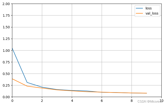
45/45 [==============================] - 290s 6s/step - loss: 1.0454 - accuracy: 0.6918 - val_loss: 0.3877 - val_accuracy: 0.9242
Epoch 2/10
45/45 [==============================] - 249s 6s/step - loss: 0.3091 - accuracy: 0.9469 - val_loss: 0.2299 - val_accuracy: 0.9545
······
Epoch 9/10
45/45 [==============================] - 276s 6s/step - loss: 0.0827 - accuracy: 0.9879 - val_loss: 0.0839 - val_accuracy: 0.9848
Epoch 10/10
45/45 [==============================] - 277s 6s/step - loss: 0.0779 - accuracy: 0.9860 - val_loss: 0.0797 - val_accuracy: 0.9848
4张图片


以及只训练最后五层的样例:
# 只保留最后五层训练,其他全部冻结 这个就不训练了,太久了 给出使用样例
resnet50 = keras.applications.ResNet50(include_top = False,pooling = 'avg',weights = 'imagenet')
#设置只有最后的5层可以训练
for layer in resnet50.layers[0:-5]:
    layer.trainable = False
resnet50_new = keras.models.Sequential([
    resnet50,
    keras.layers.Dense(num_classes, activation = 'softmax'),
])
resnet50_new.compile(loss="categorical_crossentropy",optimizer="sgd", metrics=['accuracy'])
resnet50_new.summary()
输出:
Model: "sequential_5"
_________________________________________________________________
 Layer (type)                Output Shape              Param #
=================================================================
 resnet50 (Functional)       (None, 2048)              23587712

 dense_5 (Dense)             (None, 10)                20490

=================================================================
Total params: 23608202 (90.06 MB)
Trainable params: 1075210 (4.10 MB)
Non-trainable params: 22532992 (85.96 MB)
_________________________________________________________________
Epoch 1/10
45/45 [==============================] - 276s 6s/step - loss: 0.9420 - accuracy: 0.7533 - val_loss: 0.3512 - val_accuracy: 0.9280
Epoch 2/10
45/45 [==============================] - 249s 6s/step - loss: 0.2985 - accuracy: 0.9553 - val_loss: 0.1910 - val_accuracy: 0.9583
······
Epoch 9/10
45/45 [==============================] - 284s 6s/step - loss: 0.0800 - accuracy: 0.9870 - val_loss: 0.0818 - val_accuracy: 0.9811
Epoch 10/10
45/45 [==============================] - 293s 6s/step - loss: 0.0793 - accuracy: 0.9870 - val_loss: 0.0690 - val_accuracy: 0.9886
图片见下


关键的源码分析
实际上就是要对于残差块进行理解,特别是填补0,这种做法:
#下面是残差块,因为resnet是一个一个残差块
def residual_block(x, output_channel):
    """residual connection implementation"""
    input_channel = x.get_shape().as_list()[-1] #这个是输入通道数
    #如果输出通道是输入通道的两倍,因为输出通道的数目增加了,所以需要增加维度,increase_dim = True
    if input_channel * 2 == output_channel:
        increase_dim = True
        strides = (2, 2)
    elif input_channel == output_channel:#如果输入通道和输出通道一致,图像大小不变,increase_dim是False
        increase_dim = False
        strides = (1, 1)
    else:
        raise Exception("input channel can't match output channel")
    #接着根据图形经过两个卷积层,经过两个卷积层,输出大小变为1半,大小和通道数是两码事
    conv1 = tf.layers.conv2d(x,output_channel,(3,3),strides = strides,padding = 'same',activation = tf.nn.relu,name = 'conv1')
    conv2 = tf.layers.conv2d(conv1,output_channel,(3, 3),strides = (1, 1),padding = 'same',activation = tf.nn.relu,name = 'conv2')
    if increase_dim:#如果通道数增加,就做平均值池化
        # [None, image_width, image_height, channel] -> [,,,channel*2]
        pooled_x = tf.layers.average_pooling2d(x,(2, 2),(2, 2),padding = 'valid')  #这里平均值和最大值池化都可以选
        #因为前面3维是样本数,宽,高,维度不变,最后一维通道左右各增加一半,比如原来通道是32,现在再32,就是64
        #就可以相加
        padded_x = tf.pad(pooled_x,[[0,0],[0,0],[0,0],[input_channel // 2, input_channel // 2]])
    else:
        padded_x = x  #不increase_dim,保持最初不变,直接相加
    output_x = conv2 + padded_x  #这里就是残差连接的基本结构,padded_x就是图中直连的那条线 这个就是重点的残差
    return output_x
InceptionNet
参考链接链接
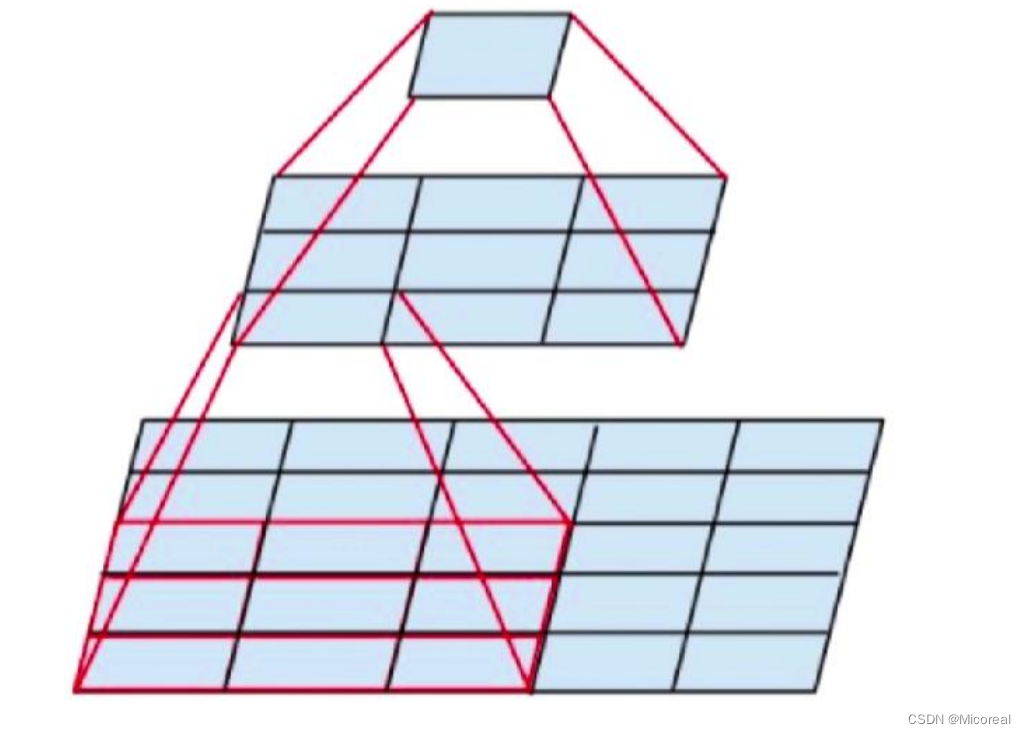
InceptionNet是CNN分类器发展的重要里程碑。在它诞生之前,为了能够获得更好的性能,大多数流行的CNN只是将卷积层叠加得越来越深,但是在出现这个之后,类似之前介绍的深度可分离卷积,这边采用的方式就是使用一定的宽度替代上深度。
支持的原理:由于信息位置的巨大变化(不同的图片当中,对应需要检测的图片比如猫的大小往往有着差距,有的很大,有的很小),为卷积操作选择正确的内核大小变得困难。大内核有益于捕获全局信息,而更小的内核有利于获取局部信息。非常深的网络容易过度拟合。它也很难通过整个网络传递梯度更新。简单地堆叠大卷积运算在计算上是昂贵的。
所以就有了第一版本的分组卷积,我们拿不同的卷积去卷一张图,最后再按照通道累加起来,形成一个通道更多的图片,也即我们对于这张照片的不同视角,从而替代之前更深的操作。
下面是V1版本的InceptionNet,这边给出的代码实现也主要和V1版本的相关,其他的实现方式也相类似,这边就不多进行解释:
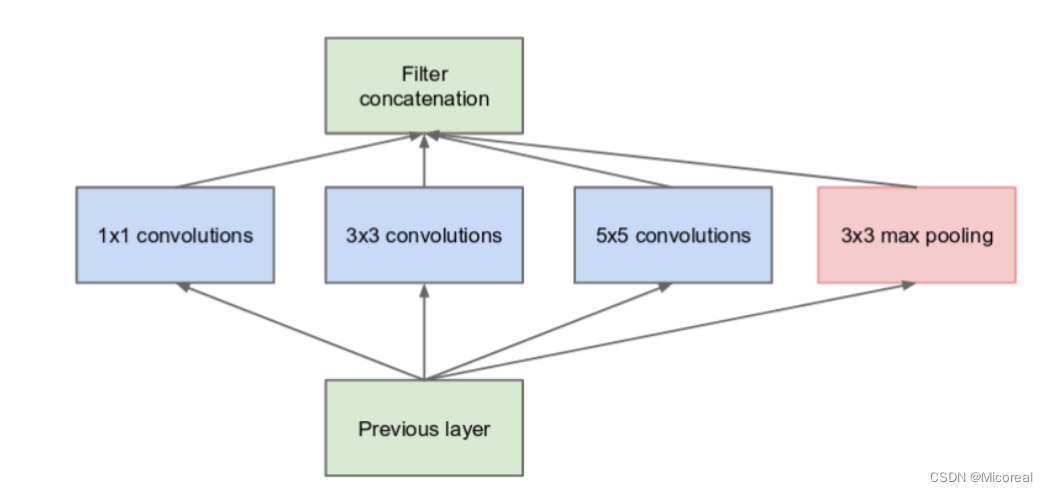
重点的代码就是这一个块:
def inception_block(x,output_channel_for_each_path,name):
    """inception block implementation"""
    """
    Args:
    - x:
    - output_channel_for_each_path: 要求输出的每一个分支的通道数 [10, 20, 5]
    - name:
    """
    with tf.variable_scope(name): #使用scope可以防止命名冲突
        conv1_1 = tf.layers.conv2d(x,output_channel_for_each_path[0],(1, 1),strides = (1,1),padding = 'same',activation = tf.nn.relu, name = 'conv1_1')
        conv3_3 = tf.layers.conv2d(x,output_channel_for_each_path[1],(3, 3),strides = (1,1),padding = 'same',activation = tf.nn.relu,name = 'conv3_3')
        conv5_5 = tf.layers.conv2d(x,output_channel_for_each_path[2],(5, 5),strides = (1,1),padding = 'same',activation = tf.nn.relu,name = 'conv5_5')
        max_pooling = tf.layers.max_pooling2d(x,(2, 2),(2, 2),name = 'max_pooling')

    max_pooling_shape = max_pooling.get_shape().as_list()[1:]  #因为0是样本,所以1后面取出的是输出大小
    input_shape = x.get_shape().as_list()[1:] #输入大小
    width_padding = (input_shape[0] - max_pooling_shape[0]) // 2 #padding的size参考文档中的表格图
    height_padding = (input_shape[1] - max_pooling_shape[1]) // 2
    padded_pooling = tf.pad(max_pooling,[[0, 0],[width_padding, width_padding],[height_padding, height_padding],[0, 0]])  #宽度和高度都做了padding,因为max_pooling后变为一半,补上才能够做concat
    concat_layer = tf.concat([conv1_1, conv3_3, conv5_5, padded_pooling],axis = 3)#0轴是样本数,1,2轴是size相同,通道数增加
    return concat_layer
这边好好理解一下,实际上和之前的深度可分离卷积是一致的。
然后最后一个总结,就是关于卷积的总结小测试,我们来计算出卷积每一步的shape:
x = tf.placeholder(tf.float32, [None, 3072])
y = tf.placeholder(tf.int64, [None])
# [None], eg: [0,5,6,3]
x_image = tf.reshape(x, [-1, 3, 32, 32])
# 32*32
x_image = tf.transpose(x_image, perm=[0, 2, 3, 1])

# conv1: 神经元图, feature_map, 输出图像
conv1 = tf.layers.conv2d(x_image,
                         32, # output channel number
                         (3,3), # kernel size
                         padding = 'same',
                         activation = tf.nn.relu,
                         name = 'conv1')

pooling1 = tf.layers.max_pooling2d(conv1,
                                   (2, 2), # kernel size
                                   (2, 2), # stride
                                   name = 'pool1')
#每次做两次inception_block后,做一次pooling处理
inception_2a = inception_block(pooling1,
                               [16, 16, 16],
                               name = 'inception_2a')  #上面封装好的3层卷积加一层池化
print(inception_2a.shape)
inception_2b = inception_block(inception_2a,
                               [16, 16, 16],
                               name = 'inception_2b')
print(inception_2b.shape)
pooling2 = tf.layers.max_pooling2d(inception_2b,
                                   (2, 2), # kernel size
                                   (2, 2), # stride
                                   name = 'pool2')

inception_3a = inception_block(pooling2,
                               [16, 16, 16],
                               name = 'inception_3a')
print(inception_3a.shape)
inception_3b = inception_block(inception_3a,
                               [16, 16, 16],
                               name = 'inception_3b')
print(inception_3b.shape)
pooling3 = tf.layers.max_pooling2d(inception_3b,
                                   (2, 2), # kernel size
                                   (2, 2), # stride
                                   name = 'pool3')

print(pooling3.shape)
flatten = tf.layers.flatten(pooling3)
y_ = tf.layers.dense(flatten, 10)
输出:
(?, 16, 16, 80)
(?, 16, 16, 128)
(?, 8, 8, 176)
(?, 8, 8, 224)
(?, 4, 4, 224)


 3546
3546


 被折叠的 条评论
为什么被折叠?
被折叠的 条评论
为什么被折叠?
 到【灌水乐园】发言


