


之前总结过 R N N L M RNNLM RNNLM,是一个SequenceModel,其结构类似如下:

这里面是一个一个的输出。我们如果以这种方式做机器翻译,每一个时刻输入一个词,相应的翻译一个词,显然这种一个一个单词的翻译方式不是很好,因为没有联系上下文进行翻译。我们希望先把一整句话喂给模型,然后模型在这一个整句的角度上来进翻译。这样翻译的效果更好。
所以本篇博文要总结的是Seq2Seq Model,给出一个完整的句子,能得出另外一个完整的句子。
下面我们以机器翻译来讲解下面几个要点。
Encoder-Decoder模型
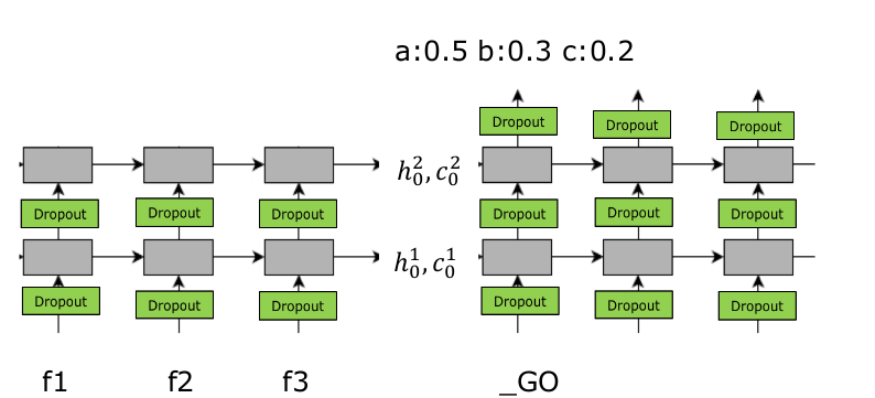
网络结构
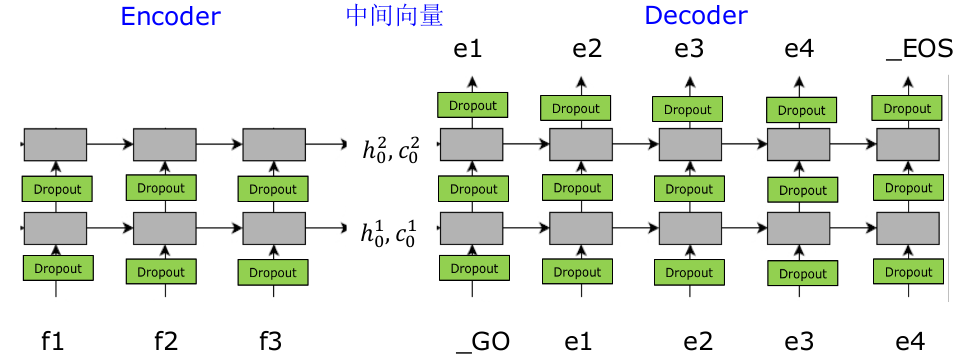
其中 f 1 , f 2 , f 3 {f}_{1},{f}_{2},{f}_{3} f1,f2,f3 是输入信息做完 e m b e d d i n g embedding embedding 后的矩阵,Encoder部分是一个两层的 L S T M LSTM LSTM 神经网络,这个神经网络不做任何输出,只输出最后一步的 h , c h,c h,c,我们可以理解这个 h , c h,c h,c 是已经总结了的输入信息, D e c o d e r 部 分 Decoder部分 Decoder部分也是一个两层的 L S T M LSTM LSTM 神经网络,并且其隐藏层 h , c h,c h,c 的初始值为 E n c o d e r Encoder Encoder 部分输出的 h , c h,c h,c,然后在 D e c o d e r Decoder Decoder 部分进行翻译。
注意在 E n c o d e r Encoder Encoder 部分每一步并不预测任何东西,其初始的 h , c h,c h,c 为全零向量,并且与 D e c o d e r Decoder Decoder 是完全不同的参数。
### E n c o d e r − D e c o d e r Encoder-Decoder Encoder−Decoder 的参数集合
首先注意 E n c o d e r Encoder Encoder 和 D e c o d e r Decoder Decoder 部分都是两层的 L S T M LSTM LSTM 神经网络。回顾下 L S T M C e l l LSTM\ Cell LSTM Cell 大致结构:

以及它的计算公式:

E n c o d e r − D e c o d e r Encoder-Decoder Encoder−Decoder 超参数
- n u m _ l a y e r s = n , h i d d e n s i z e = d ( e m b e d d i n g 的 维 度 ) num\_layers=n, hidden\ size=d(embedding的维度) num_layers=n,hidden size=d(embedding的维度)
- v o c a b f o r F = V F ( 输 入 单 词 的 个 数 ) , v o c a b f o r E = V E ( 输 出 单 词 的 个 数 ) vocab\ for\ F = {V}_{F}(输入单词的个数) , vocab\ for\ E = {V}_{E}(输出单词的个数) vocab for F=VF(输入单词的个数),vocab for E=VE(输出单词的个数)
E n c o d e r Encoder Encoder 部分参数
- I n p u t : i n p u t e m b e d d i n g f o r f : V F ∗ d Input: input\ embedding\ for\ f : {V}_{F} ∗ d Input:input embedding for f:VF∗d
- L S T M LSTM LSTM: 第一层,第二层: 2 ∗ ( 8 d 2 + 4 d ) 2*(8{d}^{2} +4d) 2∗(8d2+4d)(我们可以看上面 L S T M LSTM LSTM 的计算公式,对于 i , f , o , g i,f,o,g i,f,o,g 四个公式,每个公式都有两个参数矩阵,每个矩阵大小都是 d ∗ d d*d d∗d,再加上四个 b i a s bias bias 参数矩阵,故每层共有 ( 8 d 2 + 4 d ) (8{d}^{2} +4d) (8d2+4d) 个参数)
D e c o d e r Decoder Decoder 部分参数
- I n p u t : i n p u t e m b e d d i n g f o r e : V E ∗ d Input: input\ embedding\ for\ e: {V}_{E} ∗ d Input:input embedding for e:VE∗d
- L S T M LSTM LSTM: 第一层,第二层: 2 ∗ ( 8 d 2 + 4 d ) 2*(8{d}^{2} +4d) 2∗(8d2+4d)
-
O
u
t
p
u
t
Output
Output
o u t p u t e m b e d d i n g f o r e : V E ∗ d output\ embedding\ for\ e: {V}_{E} ∗ d output embedding for e:VE∗d
o u t p u t b i a s f o r e : V E output\ bias\ for\ e: {V}_{E} output bias for e:VE
Beam Search
M i s m a t c h b e t w e e n T r a i n a n d T e s t Mismatch\ between\ Train\ and\ Test Mismatch between Train and Test
首先需要注意到模型训练和模型预测是两个不同的过程,在训练时,我们知道每一步真正的 r e f e r e n c e reference reference,而在预测时是不知道每一步的 r e f e r e n c e reference reference 的。
在上图的网络结构中,都是以上一时刻真正的 r e f e r e n c e reference reference 作为下一时刻的 i n p u t input input 来训练模型。
那么 t r a i n train train 出这样一个模型,应该如何进行预测呢?因为在预测阶段我们是不知道 r e f e r e n c e reference reference 的,我们可以尝试这样做,把上一次的输出作为下一次的输入。
很显然,这样做的后果很严重:

一步错,步步错!
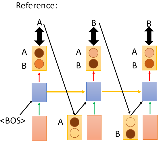
那么应如何解决上面这个问题呢?我们尝试这样做,现在假设语料库只有 A , B A,B A,B 两个 w o r d word word,那么:
我们看上图的 L S T M LSTM LSTM 结构,共有三个时间段,第一个时间段会输出两个单词 P ( A ) , P ( B ) P(A),P(B) P(A),P(B) 的概率,并不真正的输出最大概率对应的 w o r d word word 作为当时刻的输出,分别以 [ A , B ] T {[A,B]}^{T} [A,B]T 作为下一个时刻的输入,然后得到这一时刻输出 P ( A ) , P ( B ) , P ( A ) , P ( B ) P(A),P(B),P(A),P(B) P(A),P(B),P(A),P(B) 的概率矩阵,以此类推,直到最后我们可以得到输出是 A A A , A A B , A B A , A B B , . . . . . AAA,AAB,ABA,ABB,..... AAA,AAB,ABA,ABB,.....各个序列的概率,选择概率最大的作为真正的输出序列。
这里需要注意,在 D e c o d e r Decoder Decoder 部分,第三个时间步处两个输入的 B B B 表示不同的含义,第一个 B B B 的前驱为 A A A,第二个 B B B 的前驱为 B B B。
这样我们可以计算出输出序列 P ( A A A ) = 0.6 ∗ 0.4 ∗ 0.5 = 0.12 , P ( A A B ) = 0.6 ∗ 0.4 ∗ 0.5 = 0.12 , P ( A B A ) = 0.6 ∗ 0.6 ∗ 0.4 = 0.144.... P(AAA)=0.6*0.4*0.5=0.12,P(AAB)=0.6*0.4*0.5=0.12,P(ABA)=0.6*0.6*0.4=0.144.... P(AAA)=0.6∗0.4∗0.5=0.12,P(AAB)=0.6∗0.4∗0.5=0.12,P(ABA)=0.6∗0.6∗0.4=0.144.... 如此类推计算,可以计算出最大概率对应的序列,作为预测结果。
在语料库中的 w o r d s words words 很少的情况下,可以利用这样类似于穷举的方式来获得概率最大的那个序列作为预测结果,但是如果语料库中的 w o r d s words words 很多时,这种穷举的方式肯定就变得不可行了,那么这个时候应该如何做呢?
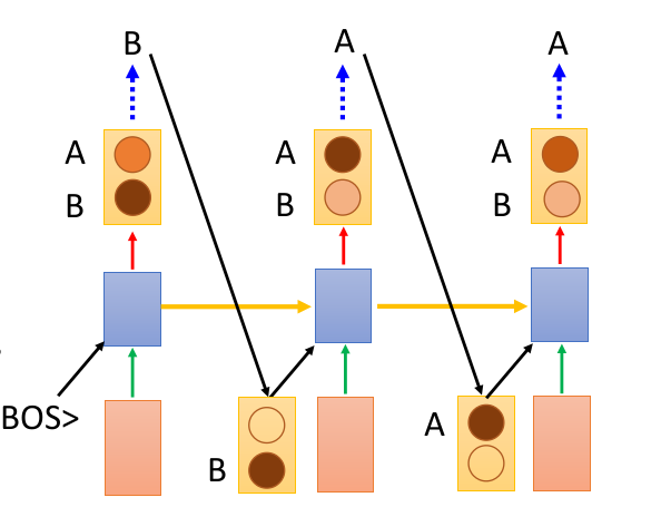
可以尝试这样做,例如语料库有3个 w o r d s words words,我们可以设置 B e a m s i z e = 2 Beam\ size = 2 Beam size=2,也就是每次选择前一时刻输出概率最大的前2个 w o r d s words words 作为当前的输入。

这里需要注意,当对应输入是 a , b a,b a,b 时,输出最大概率的两个 w o r d word word 为 b , c b,c b,c,并且其前驱都是 a a a,那么此时以 b b b 为前驱的就丢掉了。

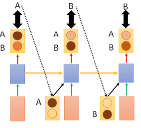
当语料库中只有两个 w o r d s words words 时,取 B e a m s i z e = 2 Beam\ size=2 Beam size=2时,其过程如下:

可以以下面这张图更好的理解 B e a m S e a r c h Beam\ Search Beam Search 过程:

注意在每个时间步时,可能有相同的 w o r d word word 作为输入,但是他们的意义是不同的,其前驱不一样。
Attention
上面讲的传统的 E n c o d e r − D e c o d e r Encoder-Decoder Encoder−Decoder 神经网络结构在应对较短文本翻译时效果不错,但是随着文本长度的增加,其翻译效果会迅速的恶化。由此提出了 A t t e n t i o n Attention Attention 这种结构,使得模型能够学习如何对 i n p u t input input 和 o u t p u t output output 进行对齐。
简单来说,例如将“我 爱 你”翻译成 " i l o v e y o u " "i\ love\ you" "i love you",这里模型如何学习到如何将翻译出的 " i " "i" "i" 对齐到( a t t e n t i o n attention attention) 到”我“。
例如下图:

那么问题来了,如何让模型学习对其( A t t e n t i o n Attention Attention) 呢?
在 a t t e n t i o n attention attention 的原始论文中是这样说的:

这里我久不从数学公式角度来说明,只说下它的大致思路。
上图中上半部分为 D e c o d e r Decoder Decoder ,其中 s s s 为其 h i d d e n − s t a t e s hidden-states hidden−states 输出信息, y y y 为其 o u t p u t output output 。下半部分为 E n c o d e r Encoder Encoder , X X X 为其 I n p u t Input Input, h h h 为 h i d d e n − s t a t e s hidden-states hidden−states 。
假设在 t t t 时刻,其 D e c o d e r Decoder Decoder 部分对应的 h i d d e n − s t a t e s hidden-states hidden−states 为 S t {S}_{t} St ,这个时候,我们把 S t {S}_{t} St 与 E n c o d e r Encoder Encoder 部分的所有 h i d d e n − s t a t e hidden-state hidden−state 信息做个相似度的计算,得出 a t , 1 , a t , 2 , a t , 3 , . . . {a}_{t,1},{a}_{t,2},{a}_{t,3},... at,1,at,2,at,3,...,然后再把这些计算出来的相似度做个 s o f t m a x softmax softmax,再进行如下计算:

将得出的 c j {c}_{j} cj 作为 D e c o d e r Decoder Decoder 部分的输入。
这样讲的估计有许多人没明白咋回事,为什么这样做就能 A t t e n t i o n Attention Attention 呢?
我觉得这篇原始论文讲的虽然详细但是不够直观。我引用下台大李宏毅教授所讲 a t t e n t i o n attention attention 的 p p t ppt ppt 来详细进行讲解。

假设我们再 E n c o d e r Encoder Encoder 部分输入“机器学习" 四个字,经过 w o r d − E m b e d d i n g word-Embedding word−Embedding 以后作为输入喂给一个 R N N RNN RNN ,然后经过隐藏层得出隐藏层信息 h 1 , h 2 , . . . {h}_{1},{h}_{2},... h1,h2,...,这时候在 D e c o d e r Decoder Decoder 部分的第一个时刻的 h i d d e n − s t a t e hidden-state hidden−state 假设为 z 0 {z}_{0} z0, z 0 {z}_{0} z0 的和 h 1 , h 2 , , , {h}_{1},{h}_{2},,, h1,h2,,,进行相似度的计算,得出各个时刻的 a 0 1 , a 0 2 , . . . {a}^{1}_{0},{a}^{2}_{0},... a01,a02,...,然后在 a i {a}^{i} ai 与对应的 h i {h}^{i} hi 相乘求和得到这 c 0 {c}_{0} c0 ,其大致过程如下:


我们可以看出 e n c o d e r encoder encoder 和 d e c o d e r decoder decoder 是联合的进行训练,在训练过程中,在某个时刻模型会学习到当前应该 f o c u s focus focus 到 i n p u t input input 的哪一部分,这体现在 a 0 1 , a 0 2 , . . . {a}^{1}_{0},{a}^{2}_{0},... a01,a02,... 不同的系数权重上, a t t e n t i o n attention attention 就是在学习这些系数。
得出的 C 0 {C}_{0} C0 作为 D e c o d e r Decoder Decoder 的下一时刻的输入。后面的时刻同理。

其实对于 a t t e n t i o n attention attention 没有固定的套路,例如 s o f t m a x softmax softmax 这一步不一定非要做,听说有人做实验发现不做 s o f t m a x softmax softmax 效果还好些。其变种有很多。


 954
954

 被折叠的 条评论
为什么被折叠?
被折叠的 条评论
为什么被折叠?
 到【灌水乐园】发言


