Classification and Representation

Classification and Representation

Classification

• $y\in${0,1}

  0:“Negative Class”

  1:“Positive Class”

  The training set is classified arbitrarily as 0 or 1.

  classification is not actually a linear function

  binary classification problem

  • y can take on only two values, 0 and 1

    Logistic Regression

    $0\le h_{\theta }(x)\le 1$

Hypothesis Representation

• Doesn’t make sense for $h_{\theta }(x)$ to take values larger than 1 or smaller than 0 when we know that y ∈ {0, 1}.

$\Rightarrow$ change the form for our hypotheses $h_{\theta }(x)$ to satisfy $0\le h_{\theta }(x)\le 1$.( by plugging ${\theta }^{T}x$ into the Logistic Function)

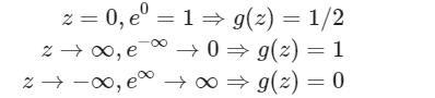
Sigmoid Function(Logistic Function)

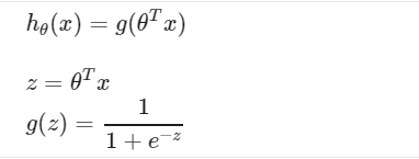
The sigmoid function looks like:

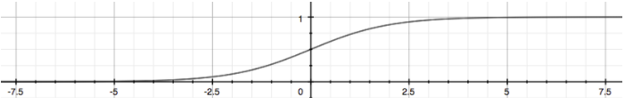
The function g(z) shown here maps any real number to the (0, 1) interval, making it useful for transforming an arbitrary-valued function into a function better suited for classification.

$h_{\theta }(x)$ will give us the probability that our output is 1.

Decision Boundary

decision boundary :

The line that separates the area where y = 0 and where y = 1. It is created by our hypothesis function.

To get our discrete 0 or 1 classification:

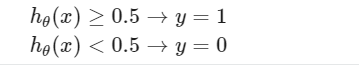
And

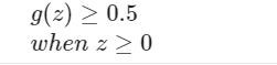
Remember:

The decision boundary is a property not of the training set, but of the hypothesis and of the parameters.

So as long as we’ve given the parameter vector $\theta$, that is what defines the decision boundary.

the parameter vector $\theta$, that is what defines the decision boundary.

The training set may be used to fit the parameters $\theta$.