第P6周：好莱坞明星识别

Nobody33

已于 2023-11-18 13:53:17 修改

阅读量65

点赞数

分类专栏： pytorch 文章标签：深度学习

于 2023-09-15 15:57:13 首次发布

本文链接：https://blog.csdn.net/S153580/article/details/132904494

版权

pytorch 专栏收录该内容

9 篇文章 0 订阅

订阅专栏

🍨 本文为🔗365天深度学习训练营中的学习记录博客

🍦 参考文章：Pytorch实战 | 第P6周：好莱坞明星识别
🍖 原作者：K同学啊 | 接辅导、项目定制
🚀 文章来源：K同学的学习圈子

一、前期准备

1、设置GPU

import torch
import torch.nn as nn
import torchvision.transforms as transforms
import torchvision
from torchvision import transforms, datasets
import os,PIL,pathlib,warnings

warnings.filterwarnings("ignore")             #忽略警告信息

device = torch.device("cuda" if torch.cuda.is_available() else "cpu")
device

关于忽略警告信息这一行，我在想为什么要设置一个“ignore”，有警告不看看？然后查资料发现是因为python有时会将能运行的代码报错，然后我想起来平时用pycharm时，确实会有很多那种黄色的小三角警告符显示“weak warning”,但是程序在运行后也没有错误，确实是可以ignore一下

device(type=‘cuda’)

2、导入数据

import os,PIL,random,pathlib

data_dir = './48-data/'
data_dir = pathlib.Path(data_dir)

data_paths  = list(data_dir.glob('*'))
classeNames = [str(path).split("\\")[1] for path in data_paths]
classeNames

[‘Angelina Jolie’,
‘Brad Pitt’,
‘Denzel Washington’,
‘Hugh Jackman’,
‘Jennifer Lawrence’,
‘Johnny Depp’,
‘Kate Winslet’,
‘Leonardo DiCaprio’,
‘Megan Fox’,
‘Natalie Portman’,
‘Nicole Kidman’,
‘Robert Downey Jr’,
‘Sandra Bullock’,
‘Scarlett Johansson’,
‘Tom Cruise’,
‘Tom Hanks’,
‘Will Smith’]

train_transforms = transforms.Compose([ #compose将transforms的一系列方法进行包装，我们调用这个以进行依次有序地对数据进行处理。transforms模块包含了一系列的图像处理方法，数据的标准化、中心化、旋转、翻转等，都是为了增强数据，增强模型的泛化能力。
    transforms.Resize([224, 224]),  # 这里开始数据预处理了，对于深度学习来说，数据的量和分布很重要。
    # transforms.RandomCrop（  ，padding=  ）#这是我在查阅Compose时另外查到的一个处理模块，它是将图片进行随机裁剪。
    transforms.ToTensor(),          # 将PIL Image或numpy.ndarray转换为tensor，并归一化到[0,1]之间
    # transforms.RandomHorizontalFlip(), # 随机水平翻转，之前我不理解这个的作用，其实这些都是数据处理的一些方法罢了，毕竟现实识别时实际情况与标准数据差别很大，这些工具的存在也是很有必要的。
    transforms.Normalize(           # 标准化处理-->转换为标准正太分布（高斯分布），使模型更容易收敛
        mean=[0.485, 0.456, 0.406], 
        #在送入网络之前将图片减去均值，消除公共部分，凸显特征和差异。
        std=[0.229, 0.224, 0.225])  # 这里我之前在想为什么平均值和标准差这里的数值一直都是一样的，然后查到这里是运用的imagenet的均值和标准差，他们是通过几百万张图片总结出来的数字，对很多图像处理模型都适用。
])

total_data = datasets.ImageFolder("./48-data/",transform=train_transforms)
total_data

Dataset ImageFolder
Number of datapoints: 1800
Root location: ./48-data/
StandardTransform
Transform: Compose(
Resize(size=[224, 224], interpolation=bilinear, max_size=None, antialias=None)
ToTensor()
Normalize(mean=[0.485, 0.456, 0.406], std=[0.229, 0.224, 0.225])
)

total_data.class_to_idx #将类别名称化为索引，以便模型的训练和预测。

{‘Angelina Jolie’: 0,
‘Brad Pitt’: 1,
‘Denzel Washington’: 2,
‘Hugh Jackman’: 3,
‘Jennifer Lawrence’: 4,
‘Johnny Depp’: 5,
‘Kate Winslet’: 6,
‘Leonardo DiCaprio’: 7,
‘Megan Fox’: 8,
‘Natalie Portman’: 9,
‘Nicole Kidman’: 10,
‘Robert Downey Jr’: 11,
‘Sandra Bullock’: 12,
‘Scarlett Johansson’: 13,
‘Tom Cruise’: 14,
‘Tom Hanks’: 15,
‘Will Smith’: 16}

3、划分数据集

train_size = int(0.8 * len(total_data)) #这里我尝试改过，从0.7到0.9，发现效果都不是很好，应该百分十八十的量九十比较好的训练集比例了。
test_size  = len(total_data) - train_size
train_dataset, test_dataset = torch.utils.data.random_split(total_data, [train_size, test_size])#pytorch里的随机分化数据集的函数，刚刚查到这个效果相当于设置随机种子
"""昨天晚上我提问的时候有人告诉我我的准确率波动可能是种子没设置，我还现查了种子是什么东西，
然后查怎么设定种子，但是看了一大篇回答一头雾水。
"""
train_dataset, test_dataset

(<torch.utils.data.dataset.Subset at 0x2570a8b6680>,
<torch.utils.data.dataset.Subset at 0x2570a8b67a0>)

batch_size = 1
"""
我在开始尝试怎么做才能优化准确率的时候，搜到增大batch_size可以增大准确率，结果就在
那里增加，然后等。结果发现根本没用。然后我意识到这是一个整体我，我仅仅这样改一个是
没有办法直接得到优化结果的。然后我查到batch就是相当于把数据分成多少份，batch_size
就是每份的大小。要想增加准确率其实该减小batch_size。这样增加了运算次数，延长了运算
时间。提高batch_size主要还是提高效率，提升GPU使用效率而已。
"""
train_dl = torch.utils.data.DataLoader(train_dataset,
                                           batch_size=batch_size,
                                           shuffle=True,
"""
我查到的shuffer=Ture表示在每一次epoch中都打乱所有数据的顺序，然后以batch为单位从头
到尾按顺序取用数据。这样的结果就是不同epoch中的数据都是乱序的。刚刚又查到就是在这里
设置随机种子就能使每一次运行的数据是乱的，但是不同次之间都是一样的乱序，感觉就是这里
了，之后好好试试。
"""
                                           num_workers=1)
test_dl = torch.utils.data.DataLoader(test_dataset,
                                          batch_size=batch_size,
                                          shuffle=True,
                                          num_workers=1)

for X, y in test_dl:
    print("Shape of X [N, C, H, W]: ", X.shape)#打印检查设置的参数，好接下来喂到模型里面。
    print("Shape of y: ", y.shape, y.dtype)
    break

Shape of X [N, C, H, W]: torch.Size([1, 3, 224, 224])
Shape of y: torch.Size([1]) torch.int64

二、调用官方的VGG-16模型

from torchvision.models import vgg16

device = "cuda" if torch.cuda.is_available() else "cpu"
print("Using {} device".format(device))
    
# 加载预训练模型，并且对模型进行微调
model = vgg16(pretrained = True).to(device) # 加载预训练的vgg16模型

for param in model.parameters():
    param.requires_grad = False # 冻结模型的参数，这样子在训练的时候只训练最后一层的参数

# 修改classifier模块的第6层（即：(6): Linear(in_features=4096, out_features=2, bias=True)）
# 注意查看我们下方打印出来的模型
model.classifier._modules['6'] = nn.Linear(4096,len(classeNames)) # 修改vgg16模型中最后一层全连接层，输出目标类别个数
model.to(device)  
model

之前专门找了卷积和池化的知识点看，感觉大致懂了。但是将他们合并起来过后我就有点懵了。卷积是通过卷积核和权重将图片特征提取。我感觉就是将卷积核依次选取的部分进行一定程度的“模糊化”，好让以后识别到其他有类似的特征的图片能识别，就像人名之间重复很少，但是提取出来姓氏就能匹配到一大批相同姓氏的人，然后后面再经过平均池化啊最大池化这些再将提取出来的特征筛选，然后再全连接，就拼接成了相同姓氏的可能和你有关系的人的一个大的一维数据，我是这么理解的。但是实际上看了很多解释感觉都说的云里雾里的。最近找到一些“Pytorch学习笔记”之类标题的文章，这些就是分享他们自己的理解，我感觉看了这些感觉好了很多。

Using cuda device

VGG(
(features): Sequential(
(0): Conv2d(3, 64, kernel_size=(3, 3), stride=(1, 1), padding=(1, 1))
(1): ReLU(inplace=True)
(2): Conv2d(64, 64, kernel_size=(3, 3), stride=(1, 1), padding=(1, 1))
(3): ReLU(inplace=True)
(4): MaxPool2d(kernel_size=2, stride=2, padding=0, dilation=1, ceil_mode=False)
(5): Conv2d(64, 128, kernel_size=(3, 3), stride=(1, 1), padding=(1, 1))
(6): ReLU(inplace=True)
(7): Conv2d(128, 128, kernel_size=(3, 3), stride=(1, 1), padding=(1, 1))
(8): ReLU(inplace=True)
(9): MaxPool2d(kernel_size=2, stride=2, padding=0, dilation=1, ceil_mode=False)
(10): Conv2d(128, 256, kernel_size=(3, 3), stride=(1, 1), padding=(1, 1))
(11): ReLU(inplace=True)
(12): Conv2d(256, 256, kernel_size=(3, 3), stride=(1, 1), padding=(1, 1))
(13): ReLU(inplace=True)
(14): Conv2d(256, 256, kernel_size=(3, 3), stride=(1, 1), padding=(1, 1))
(15): ReLU(inplace=True)
(16): MaxPool2d(kernel_size=2, stride=2, padding=0, dilation=1, ceil_mode=False)
(17): Conv2d(256, 512, kernel_size=(3, 3), stride=(1, 1), padding=(1, 1))
(18): ReLU(inplace=True)
(19): Conv2d(512, 512, kernel_size=(3, 3), stride=(1, 1), padding=(1, 1))
(20): ReLU(inplace=True)
(21): Conv2d(512, 512, kernel_size=(3, 3), stride=(1, 1), padding=(1, 1))
(22): ReLU(inplace=True)
(23): MaxPool2d(kernel_size=2, stride=2, padding=0, dilation=1, ceil_mode=False)
(24): Conv2d(512, 512, kernel_size=(3, 3), stride=(1, 1), padding=(1, 1))
(25): ReLU(inplace=True)
(26): Conv2d(512, 512, kernel_size=(3, 3), stride=(1, 1), padding=(1, 1))
(27): ReLU(inplace=True)
(28): Conv2d(512, 512, kernel_size=(3, 3), stride=(1, 1), padding=(1, 1))
(29): ReLU(inplace=True)
(30): MaxPool2d(kernel_size=2, stride=2, padding=0, dilation=1, ceil_mode=False)
)
(avgpool): AdaptiveAvgPool2d(output_size=(7, 7))
(classifier): Sequential(
(0): Linear(in_features=25088, out_features=4096, bias=True)
(1): ReLU(inplace=True)
(2): Dropout(p=0.5, inplace=False)
(3): Linear(in_features=4096, out_features=4096, bias=True)
(4): ReLU(inplace=True)
(5): Dropout(p=0.5, inplace=False)
(6): Linear(in_features=4096, out_features=17, bias=True)
)
)

三、训练模型

1. 编写训练函数

# 训练循环
def train(dataloader, model, loss_fn, optimizer):
    size = len(dataloader.dataset)  # 训练集的大小
    num_batches = len(dataloader)   # 批次数目, (size/batch_size，向上取整)

    train_loss, train_acc = 0, 0  # 初始化训练损失和正确率
    
    for X, y in dataloader:  # 获取图片及其标签
        X, y = X.to(device), y.to(device)
        
        # 计算预测误差
        pred = model(X)          # 网络输出
        loss = loss_fn(pred, y)  # 计算网络输出和真实值之间的差距，targets为真实值，计算二者差值即为损失
        
        # 反向传播
        optimizer.zero_grad()  # grad属性归零
        loss.backward()        # 反向传播
        optimizer.step()       # 每一步自动更新
        
        # 记录acc与loss
        train_acc  += (pred.argmax(1) == y).type(torch.float).sum().item()
        train_loss += loss.item()
            
    train_acc  /= size
    train_loss /= num_batches

    return train_acc, train_loss

我理解的损失函数是在每一次正向传播完了过后倒过来反向传播时，评判前一次正向传播好不好的东西。我感觉我能理解损失函数的原理，就是到了代码这里想不明白到底是怎么进行评估的，看了很多回答，有一种似懂非懂的感觉。

2.编写测试函数

def test (dataloader, model, loss_fn):
    size        = len(dataloader.dataset)  # 测试集的大小
    num_batches = len(dataloader)          # 批次数目, (size/batch_size，向上取整)
    test_loss, test_acc = 0, 0
    
    # 当不进行训练时，停止梯度更新，节省计算内存消耗
    with torch.no_grad():
        for imgs, target in dataloader:
            imgs, target = imgs.to(device), target.to(device)
            
            # 计算loss
            target_pred = model(imgs)
            loss        = loss_fn(target_pred, target)
            
            test_loss += loss.item()
            test_acc  += (target_pred.argmax(1) == target).type(torch.float).sum().item()

    test_acc  /= size
    test_loss /= num_batches

    return test_acc, test_loss

3. 设置动态学习率

learn_rate = 1e-6

这个东西我好好看了，因为都说这个很重要。我现在掌握的概念是学习率相当于一种探测，它在那个函数两侧跳来跳去不断向下知道最低谷也就是最优值，学习率大了会一直反复横跳，难以下降到谷底，相当于步子跨大了，老是把那个最优值给跨过去。但是学习率过于小有导致步子太小，效率底下。这里之前我想的是我设的足够小大不了就是运算时间长一点罢了，但是我实际运算发现过分小了过后还是会有准确率在每一个epoch之间波动特别大的问题，而且越小越离谱，这个目前我还没想明白为什么。

# 调用官方动态学习率接口时使用
lambda1 = lambda epoch: 0.92 ** (epoch // 4)
optimizer = torch.optim.SGD(model.parameters(), lr=learn_rate)
scheduler = torch.optim.lr_scheduler.LambdaLR(optimizer, lr_lambda=lambda1) #选定调整方法

import copy

loss_fn    = nn.CrossEntropyLoss() # 创建损失函数
epochs     = 40

train_loss = []
train_acc  = []
test_loss  = []
test_acc   = []

best_acc = 60    # 设置一个最佳准确率，作为最佳模型的判别指标

for epoch in range(epochs):
    # 更新学习率（使用自定义学习率时使用）
    # adjust_learning_rate(optimizer, epoch, learn_rate)
    
    model.train()
    epoch_train_acc, epoch_train_loss = train(train_dl, model, loss_fn, optimizer)
    scheduler.step() # 更新学习率（调用官方动态学习率接口时使用）
    
    model.eval()
    epoch_test_acc, epoch_test_loss = test(test_dl, model, loss_fn)
    
    # 保存最佳模型到 best_model
    if epoch_test_acc > best_acc:
        best_acc   = epoch_test_acc
        best_model = copy.deepcopy(model)
    
    train_acc.append(epoch_train_acc)
    train_loss.append(epoch_train_loss)
    test_acc.append(epoch_test_acc)
    test_loss.append(epoch_test_loss)
    
    # 获取当前的学习率
    lr = optimizer.state_dict()['param_groups'][0]['lr']
    
    template = ('Epoch:{:2d}, Train_acc:{:.1f}%, Train_loss:{:.3f}, Test_acc:{:.1f}%, Test_loss:{:.3f}, Lr:{:.2E}')
    print(template.format(epoch+1, epoch_train_acc*100, epoch_train_loss, 
                          epoch_test_acc*100, epoch_test_loss, lr))
    
# 保存最佳模型到文件中
PATH = './best_model.pth'  # 保存的参数文件名
torch.save(model.state_dict(), PATH)

print('Done')

我现在仔细看了这一段发现其实改这一段其实才是最最主要的，我一直以为这里是一个封装好的固定模型，我不能轻易改，但现在看来好像这里的损失函数，设置的epoch数都挺重要的。主要是以前一直都在查前面的知识。我应该改变一下思路，不能一点一点学。有时候先学后面说不定前面就懂了，感觉我现在的学习思维和能力还停留在中学，必须要手把手的教，但是后面应该会好起来的，我感觉学这个的过程中我走了超级多弯路，每天都在看从零开始学深度学习的书和文章，一直没有往前走，但是现在逐渐有了眉目了。接下来要把这些代码好好的亲手打一遍，就知道哪些可以改了。

这个图我当时测了很多次才出来，我还很高兴，想着终于通过自己的努力提高了准确率了，但是现在看来问题太多了，背后的逻辑我完全没有搞懂，但是在改这个文章的过程中我也在不断地查资料，感觉思路突然清晰了很多。果然学这些东西还是要勤上手，光看理论很难有进步。

四、结果可视化

1. Loss与Accuracy图

import matplotlib.pyplot as plt#这个是导入了python的一个库，从而能将我们训练的过程和数据通过图表的方式显示出来，便于分析和查看，我理解为matlab的同级别存在。
#隐藏警告
import warnings
warnings.filterwarnings("ignore")               #忽略警告信息
plt.rcParams['font.sans-serif']    = ['SimHei'] # 用来正常显示中文标签
plt.rcParams['axes.unicode_minus'] = False      # 用来正常显示负号
plt.rcParams['figure.dpi']         = 100        #分辨率

epochs_range = range(epochs)

plt.figure(figsize=(12, 3))
plt.subplot(1, 2, 1)

plt.plot(epochs_range, train_acc, label='Training Accuracy')
plt.plot(epochs_range, test_acc, label='Test Accuracy')
plt.legend(loc='lower right')
plt.title('Training and Validation Accuracy')
"""
这些东西就很好理解了就是设置图片大小和标题、各轴的标示等。这里学好了生成的图
也很美观，要是要是有机会发论文那么会很有帮助。
"""
plt.subplot(1, 2, 2)
plt.plot(epochs_range, train_loss, label='Training Loss')
plt.plot(epochs_range, test_loss, label='Test Loss')
plt.legend(loc='upper right')
plt.title('Training and Validation Loss')
plt.show()

PS：由于当时忘记保存，在这个准确率出来的时候我就把内核叫停了，然后拿去讨论为什么会出现准确率在每个EPOCH之间波动这么大去了，也没有用seed，后来才知道不断调参中断内核在继续本身就会对结果造成影响，现在再怎么测试也弄不出这个结果了，故而也没有这个图了。

2.指定图片进行预测

from PIL import Image 

classes = list(total_data.class_to_idx)

def predict_one_image(image_path, model, transform, classes):
    
    test_img = Image.open(image_path).convert('RGB') #转换为三通道
    plt.imshow(test_img)  # 展示预测的图片

    test_img = transform(test_img)
    img = test_img.to(device).unsqueeze(0) #扩展维度
    
    model.eval()
    output = model(img)

    _,pred = torch.max(output,1)
    pred_class = classes[pred]
    print(f'预测结果是：{pred_class}')

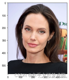
# 预测训练集中的某张照片
predict_one_image(image_path='./48-data/Angelina Jolie/001_fe3347c0.jpg', 
                  model=model, 
                  transform=train_transforms, 
                  classes=classes)

预测结果是：Angelina Jolie

3.模型评估

best_model.eval()
epoch_test_acc, epoch_test_loss = test(test_dl, best_model, loss_fn)

epoch_test_acc, epoch_test_loss

# 查看是否与我们记录的最高准确率一致
epoch_test_acc

故以下这些数据都没有了

Nobody33

关注

0
点赞
踩
0

收藏

觉得还不错? 一键收藏
0
评论
第P6周：好莱坞明星识别

我感觉就是将卷积核依次选取的部分进行一定程度的“模糊化”，好让以后识别到其他有类似的特征的图片能识别，就像人名之间重复很少，但是提取出来姓氏就能匹配到一大批相同姓氏的人，然后后面再经过平均池化啊最大池化这些再将提取出来的特征筛选，然后再全连接，就拼接成了相同姓氏的可能和你有关系的人的一个大的一维数据，我是这么理解的。我现在仔细看了这一段发现其实改这一段其实才是最最主要的，我一直以为这里是一个封装好的固定模型，我不能轻易改，但现在看来好像这里的损失函数，设置的epoch数都挺重要的。故以下这些数据都没有了。
复制链接

扫一扫