【A_star三维路径规划】基于matlab A_star算法机器人栅格地图三维路径规划【含Matlab源码 190期】

海神之光

已于 2023-10-28 12:47:14 修改

阅读量2.8k

点赞数 4

分类专栏： Matlab路径规划（进阶版）文章标签： matlab

于 2021-09-16 21:43:20 首次发布

代码事宜私信博主

本文链接：https://blog.csdn.net/TIQCmatlab/article/details/120338250

版权

Matlab路径规划（进阶版）专栏收录该内容

609 篇文章 769 订阅

订阅专栏

✅博主简介：热爱科研的Matlab仿真开发者，修心和技术同步精进，Matlab项目合作可私信。
🍎个人主页：海神之光
🏆代码获取方式：
海神之光Matlab王者学习之路—代码获取方式
⛳️座右铭：行百里者，半于九十。

⛄一、A_star算法简介

1 A Star算法及其应用现状
进行搜索任务时提取的有助于简化搜索过程的信息被称为启发信息.启发信息经过文字提炼和公式化后转变为启发函数.启发函数可以表示自起始顶点至目标顶点间的估算距离, 也可以表示自起始顶点至目标顶点间的估算时间等.描述不同的情境、解决不同的问题所采用的启发函数各不相同.我们默认将启发函数命名为H (n) .以启发函数为策略支持的搜索方式我们称之为启发型搜索算法.在救援机器人的路径规划中, A Star算法能结合搜索任务中的环境情况, 缩小搜索范围, 提高搜索效率, 使搜索过程更具方向性、智能性, 所以A Star算法能较好地应用于机器人路径规划相关领域.

2 A Star算法流程
承接2.1节, A Star算法的启发函数是用来估算起始点到目标点的距离, 从而缩小搜索范围, 提高搜索效率.A Star算法的数学公式为:F (n) =G (n) +H (n) , 其中F (n) 是从起始点经由节点n到目标点的估计函数, G (n) 表示从起点移动到方格n的实际移动代价, H (n) 表示从方格n移动到目标点的估算移动代价.

如图2所示, 将要搜寻的区域划分成了正方形的格子, 每个格子的状态分为可通过(walkable) 和不可通过 (unwalkable) .取每个可通过方块的代价值为1, 且可以沿对角移动 (估值不考虑对角移动) .其搜索路径流程如下:
在这里插入图片描述
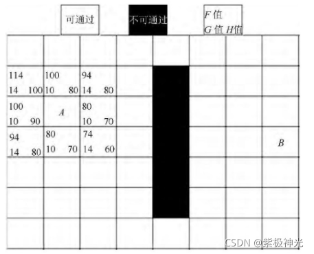
图2 A Star算法路径规划
Step1:定义名为open和closed的两个列表;open列表用于存放所有被考虑来寻找路径的方块, closed列表用于存放不会再考虑的方块;
Step2:A为起点, B为目标点, 从起点A开始, 并将起点A放入open列表中, closed列表初始化为空;
Step3:查看与A相邻的方格n (n称为A的子点, A称为n的父点) , 可通过的方格加入到open列表中, 计算它们的F, G和H值.将A从open移除加入到closed列表中;
Step4:判断open列表是否为空, 如果是, 表示搜索失败, 如果不是, 执行下一步骤;
Step5:将n从open列表移除加入到closed列表中, 判断n是否为目标顶点B, 如果是, 表示搜索成功, 算法运行结束;
Step6:如果不是, 则扩展搜索n的子顶点:
a.如果子顶点是不可通过或在close列表中, 忽略它.
b.子顶点如果不在open列表中, 则加入open列表, 并且把当前方格设置为它的父亲, 记录该方格的F, G和H值.
Step7:跳转到步骤Step4;
Step8:循环结束, 保存路径.从终点开始, 每个方格沿着父节点移动直至起点, 即是最优路径.A Star算法流程图如图3所示.
在这里插入图片描述
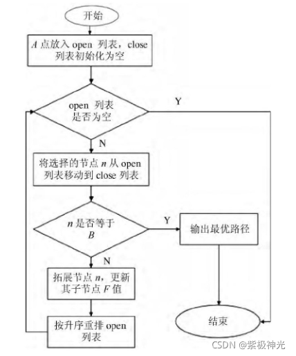
图3 A Star算法流程

⛄二、部分源代码

%Main

clc
clear

%%%%%%%%%%%%%%%%%%%%%%%%%%%%%%%%%%%%%%%%%%%%%%%%%%%%%%%%%%%%%%%%%%%%%%%%%%%
%Grid and path parameters

%Grid size [y,x,z] and resolution
sizeE=[80 80 20];
d_grid=1;

%Starting point
x0=5;
y0=7;
z0=12;

%Arrival point
xend=68;
yend=66;
zend=6;

%Number of points with low elevation around start and end point area
n_low=3;

%A* or Theta* cost weights
kg=1;
kh=1.25;
ke=sqrt((xend-x0)^2+(yend-y0)2+(zend-z0)^2);

%%%%%%%%%%%%%%%%%%%%%%%%%%%%%%%%%%%%%%%%%%%%%%%%%%%%%%%%%%%%%%%%%%%%%%%%%%%
%Map definition

%Average flight altitude
h=max(z0,zend);

%Points coordinates in [y,x,z] format
P0=[y0 x0 z0];
Pend=[yend xend zend];

%Generate map
[E,E_safe,E3d,E3d_safe]=grid_3D_safe_zone(sizeE,d_grid,h,P0,Pend,n_low);

%%%%%%%%%%%%%%%%%%%%%%%%%%%%%%%%%%%%%%%%%%%%%%%%%%%%%%%%%%%%%%%%%%%%%%%%%%%
%Path generation

%Store gains in vector
K=[kg kh ke];

%Measure path computation time
tic

%Generate path (chose one)
% [path,n_points]=a_star_3D(K,E3d_safe,x0,y0,z0,xend,yend,zend,sizeE);
% [path,n_points]=theta_star_3D(K,E3d_safe,x0,y0,z0,xend,yend,zend,sizeE);
[path,n_points]=lazy_theta_star_3D(K,E3d_safe,x0,y0,z0,xend,yend,zend,sizeE);

T_path=toc;

%Path waypoints partial distance

%Initialize
path_distance=zeros(n_points,1);

for i=2:n_points
path_distance(i)=path_distance(i-1)+sqrt((path(i,2)-path(i-1,2))^{2+(path(i,1)-path(i-1,1))}2+(path(i,3)-path(i-1,3))^2);
end

%%%%%%%%%%%%%%%%%%%%%%%%%%%%%%%%%%%%%%%%%%%%%%%%%%%%%%%%%%%%%%%%%%%%%%%%%%%
%Plot

%Map grid
x_grid=1:d_grid:sizeE(2);
y_grid=1:d_grid:sizeE(1);

%Path on safe map
figure(1)
surf(x_grid(2:end-1),y_grid(2:end-1),E_safe(2:end-1,2:end-1))
hold on
plot3(x0,y0,z0,‘gs’)
plot3(xend,yend,zend,‘rd’)
plot3(path(:,2),path(:,1),path(:,3),‘yx’)
plot3(path(:,2),path(:,1),path(:,3),‘w’)
axis tight
axis equal
view(0,90);
colorbar

%Path on standard map
figure(2)
surf(x_grid(2:end-1),y_grid(2:end-1),E(2:end-1,2:end-1))
hold on
plot3(x0,y0,z0,‘gs’)
plot3(xend,yend,zend,‘rd’)
plot3(path(:,2),path(:,1),path(:,3),‘yx’)
plot3(path(:,2),path(:,1),path(:,3),‘w’)
axis tight
axis equal
view(0,90);
colorbar

%Path height profile
figure(3)
plot(path_distance,path(:,3))
grid on
xlabel(‘Path distance’)
ylabel(‘Path height’)
%A star algorithm

function [path,n_points]=a_star_3D(K,E3d_safe,x0_old,y0_old,z0_old,xend_old,yend_old,zend_old,sizeE)

%%%%%%%%%%%%%%%%%%%%%%%%%%%%%%%%%%%%%%%%%%%%%%%%%%%%%%%%%%%%%%%%%%%%%%%%%%%
%Cost weights

kg=K(1);
kh=K(2);
ke=K(3);

%%%%%%%%%%%%%%%%%%%%%%%%%%%%%%%%%%%%%%%%%%%%%%%%%%%%%%%%%%%%%%%%%%%%%%%%%%%
%Algorithm

%If start and end points are not integer, they are rounded for the path genertion. Use of floor and ceil so they are different even if very close
x0=floor(x0_old);
y0=floor(y0_old);
z0=floor(z0_old);
xend=ceil(xend_old);
yend=ceil(yend_old);
zend=ceil(zend_old);

%Initialize

%Size of environment matrix
y_size=sizeE(1);
x_size=sizeE(2);
z_size=sizeE(3);

%Node from which the good neighbour is reached
came_fromx=zeros(sizeE);
came_fromy=zeros(sizeE);
came_fromz=zeros(sizeE);
came_fromx(y0,x0,z0)=x0;
came_fromy(y0,x0,z0)=y0;
came_fromz(y0,x0,z0)=z0;

%Nodes already evaluated
closed=[];

%Nodes to be evaluated
open=[y0,x0,z0];

%Cost of moving from start point to the node
G=Inf*ones(sizeE);
G(y0,x0,z0)=0;

%Initial total cost
F=Inf*ones(sizeE);
F(y0,x0,z0)=sqrt((xend-x0)^2+(yend-y0)2+(zend-z0)^2);

%Initialize
exit_path=0;

%While open is not empy
while isempty(open)0 && exit_path0

%Find node with minimum f in open

%Initialize
f_open=zeros(size(open,1),1);

%Evaluate f for the nodes in open
for i=1:size(open,1)
    f_open(i,:)=F(open(i,1),open(i,2),open(i,3));
end

%Find the index location in open for the node with minimum f
[~,i_f_open_min]=min(f_open);

%Location of node with minimum f in open
ycurrent=open(i_f_open_min,1);
xcurrent=open(i_f_open_min,2);
zcurrent=open(i_f_open_min,3);

point_current=[ycurrent, xcurrent, zcurrent];


%Check if the arrival node is reached
if xcurrent==xend && ycurrent==yend && zcurrent==zend
    
    %Arrival node reached, exit and generate path
    exit_path=1;
    
else
    
    %Add the node to closed
    closed(size(closed,1)+1,:)=point_current;
    
    %Remove the node from open
    i_open_keep=horzcat(1:i_f_open_min-1,i_f_open_min+1:size(open,1));
    open=open(i_open_keep,:);
    
    %Check neighbour nodes
    for i=-1:1
        for j=-1:1
            for k=-1:1                    
                
                %If the neighbour node is within grid
                if xcurrent+i>0 && ycurrent+j>0 && zcurrent+k>0 && xcurrent+i<=x_size && ycurrent+j<=y_size && zcurrent+k<=z_size
                    
                    %If the neighbour node does not belong to open and to closed

                    check_open=max(sum([ycurrent+j==open(:,1) xcurrent+i==open(:,2) zcurrent+k==open(:,3)],2));
                    check_closed=max(sum([ycurrent+j==closed(:,1) xcurrent+i==closed(:,2) zcurrent+k==closed(:,3)],2));
                    
                    if isempty(check_open)==1
                        check_open=0;
                    end
                    
                    if isempty(check_closed)==1
                        check_closed=0;
                    end

                    if check_open<3 && check_closed<3                            
                        
                        
                        %Add the neighbour node to open
                        open(size(open,1)+1,:)=[ycurrent+j, xcurrent+i, zcurrent+k];
                        
                        %Evaluate the distance from start to the current node + from the current node to the neighbour node
                        g_try=G(ycurrent,xcurrent,zcurrent)+sqrt(i^2+j^2+k^2);
                        
                        %If this distance is smaller than the neighbour distance
                        if g_try<G(ycurrent+j,xcurrent+i,zcurrent+k)
                            
                            %We are on the good path, save information
                            
                            %Record from which node the good neighbour is reached
                            came_fromy(ycurrent+j,xcurrent+i,zcurrent+k)=ycurrent;
                            came_fromx(ycurrent+j,xcurrent+i,zcurrent+k)=xcurrent;
                            came_fromz(ycurrent+j,xcurrent+i,zcurrent+k)=zcurrent;

⛄三、运行结果

在这里插入图片描述

⛄四、matlab版本及参考文献

1 matlab版本
2014a

2 参考文献
[1]马云红,张恒,齐乐融,贺建良.基于改进A*算法的三维无人机路径规划[J].电光与控制. 2019,26(10)

3 备注
简介此部分摘自互联网，仅供参考，若侵权，联系删除

🍅 仿真咨询
1 各类智能优化算法改进及应用
生产调度、经济调度、装配线调度、充电优化、车间调度、发车优化、水库调度、三维装箱、物流选址、货位优化、公交排班优化、充电桩布局优化、车间布局优化、集装箱船配载优化、水泵组合优化、解医疗资源分配优化、设施布局优化、可视域基站和无人机选址优化

2 机器学习和深度学习方面
卷积神经网络（CNN）、LSTM、支持向量机（SVM）、最小二乘支持向量机（LSSVM）、极限学习机（ELM）、核极限学习机（KELM）、BP、RBF、宽度学习、DBN、RF、RBF、DELM、XGBOOST、TCN实现风电预测、光伏预测、电池寿命预测、辐射源识别、交通流预测、负荷预测、股价预测、PM2.5浓度预测、电池健康状态预测、水体光学参数反演、NLOS信号识别、地铁停车精准预测、变压器故障诊断

3 图像处理方面
图像识别、图像分割、图像检测、图像隐藏、图像配准、图像拼接、图像融合、图像增强、图像压缩感知

4 路径规划方面
旅行商问题（TSP）、车辆路径问题（VRP、MVRP、CVRP、VRPTW等）、无人机三维路径规划、无人机协同、无人机编队、机器人路径规划、栅格地图路径规划、多式联运运输问题、车辆协同无人机路径规划、天线线性阵列分布优化、车间布局优化

5 无人机应用方面
无人机路径规划、无人机控制、无人机编队、无人机协同、无人机任务分配

6 无线传感器定位及布局方面
传感器部署优化、通信协议优化、路由优化、目标定位优化、Dv-Hop定位优化、Leach协议优化、WSN覆盖优化、组播优化、RSSI定位优化

7 信号处理方面
信号识别、信号加密、信号去噪、信号增强、雷达信号处理、信号水印嵌入提取、肌电信号、脑电信号、信号配时优化

8 电力系统方面
微电网优化、无功优化、配电网重构、储能配置

9 元胞自动机方面
交通流人群疏散病毒扩散晶体生长

10 雷达方面
卡尔曼滤波跟踪、航迹关联、航迹融合