


欢迎关注微信公众号(医学生物信息学),医学生的生信笔记,记录学习过程。
常见图片的格式包括:pdf,jpeg,tiff,png,svg,wmf。
pdf,svg和wmf为矢量图格式,放大图片时不会出现模糊。
jpeg,tiff和png为位图格式,调整文件大小时会出现模糊。
ggsave()来保存图片
通过ggplot2来绘图,那么可以使用ggsave()来保存输出图片。
plot1 <- ggplot(mtcars, aes(x = wt, y = mpg)) +
  geom_point()

# 默认输出单位为英寸,可以通过units参数来指定单位
ggsave("myplot.pdf", plot1, width = 8, height = 8, units = "cm")
另一种方式是ggplot对象不赋值为plot1,在调用ggplot()之后只调用ggsave(),它将保存最后一个ggplot对象。
使用ggsave(),不需要通过print()来打印ggplot对象,如果在创建或保存图片时出错,则无需通过dev.off()来手动关闭图形设备。还有一点需要注意,ggsave()不能用于绘制多页图。
ggplot(mtcars, aes(x = wt, y = mpg)) +
  geom_point()

ggsave("myplot.pdf", width = 8, height = 8, units = "cm")
输出图片为PDF格式
方法一
pdf("myplot.pdf", width = 4, height = 4)

plot(mtcars$wt, mtcars$mpg)
print(ggplot(mtcars, aes(x = wt, y = mpg)) + geom_point())

dev.off()
默认宽度和高度的输出单位为英寸,若想输出单位为厘米,则需通过下方代码进行转换。
# 8x8 cm
pdf("myplot.pdf", width = 8/2.54, height = 8/2.54)
方法二
plot1 <- ggplot(mtcars, aes(x = wt, y = mpg)) +
  geom_point()

# 默认输出单位为英寸,可以通过units参数来指定单位
ggsave("myplot.pdf", plot1, width = 8, height = 8, units = "cm")
输出图片为SVG格式
方法一
library(svglite)
svglite("myplot.svg", width = 4, height = 4)
plot1 <- ggplot(mtcars, aes(x = wt, y = mpg)) +
  geom_point()
print(plot1)
dev.off()
方法二
plot1 <- ggplot(mtcars, aes(x = wt, y = mpg)) +
  geom_point()
ggsave("myplot.svg", plot1, width = 8, height = 8, units = "cm")
输出图片为PNG格式
方法一
# 宽度和高度以像素为单位
png("myplot.png", width = 400, height = 400)
plot(mtcars$wt, mtcars$mpg)
dev.off()
若要输出多个图片,可以在文件名中加入%d。
png("myplot-%d.png", width = 400, height = 400)
plot(mtcars$wt, mtcars$mpg)
print(ggplot(mtcars, aes(x = wt, y = mpg)) + geom_point())
dev.off()
默认输出为每英寸72像素(ppi)。这种分辨率适合在电子屏幕上显示,而300 ppi一般用于印刷。
ppi <- 300
# 计算300 ppi下4x4英寸图像的高度和宽度(以像素为单位)
png("myplot.png", width = 4*ppi, height = 4*ppi, res = ppi)
plot(mtcars$wt, mtcars$mpg)
dev.off()
方法二
ggplot(mtcars, aes(x = wt, y = mpg)) + geom_point()

# 默认输出单位为英寸,可以通过units参数来指定单位
ggsave("myplot.png", width = 8, height = 8, unit = "cm", dpi = 300)
输出图片为TIFF格式
方法一
tiff("myplot.tiff", width = 4, height = 4, units = "cm", res = 300)
plot1 <- ggplot(mtcars, aes(x = wt, y = mpg)) +
  geom_point()
print(plot1)
dev.off()
方法二
plot1 <- ggplot(mtcars, aes(x = wt, y = mpg)) +
  geom_point()
ggsave("myplot.tiff", plot1, width = 8, height = 8, units = "cm", dpi = 300)
输出图片为WMF格式
WMF文件的创建和使用方式与PDF文件非常相似,但只能在Windows上创建。
方法一
win.metafile("myplot.wmf", width = 4, height = 4)
plot1 <- ggplot(mtcars, aes(x = wt, y = mpg)) +
  geom_point()
print(plot1)
dev.off()
方法二
plot1 <- ggplot(mtcars, aes(x = wt, y = mpg)) +
  geom_point()
ggsave("myplot.wmf", plot1, width = 8, height = 8, units = "cm")
拼图
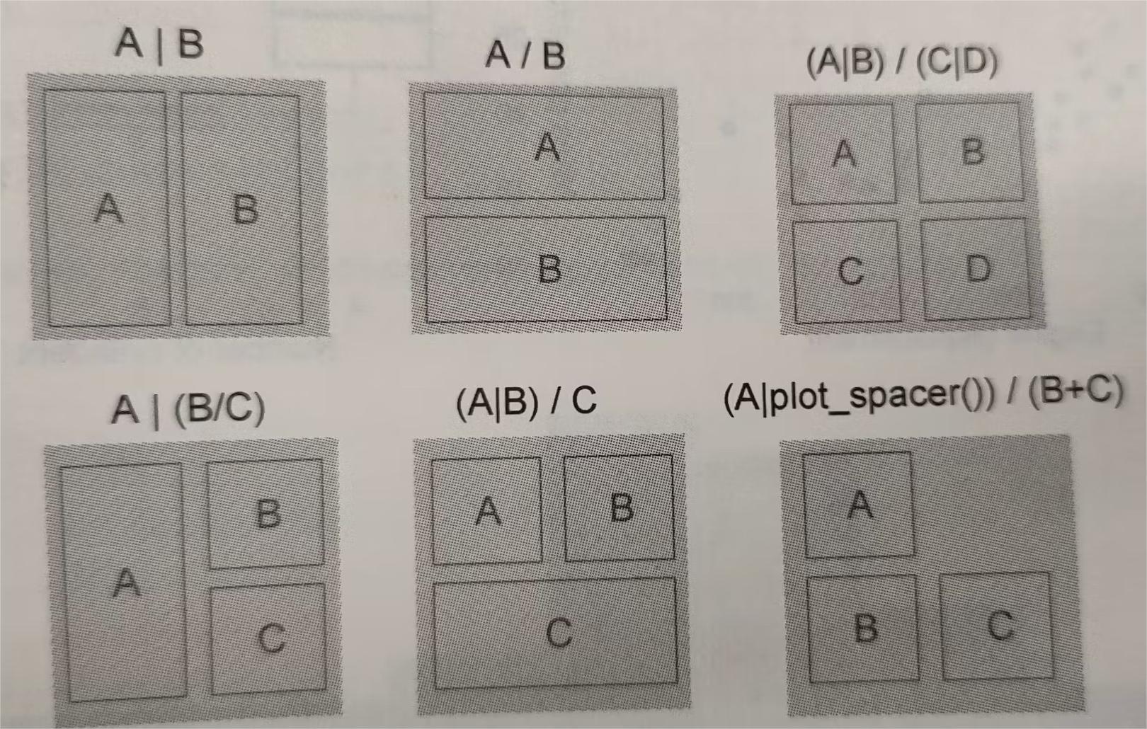
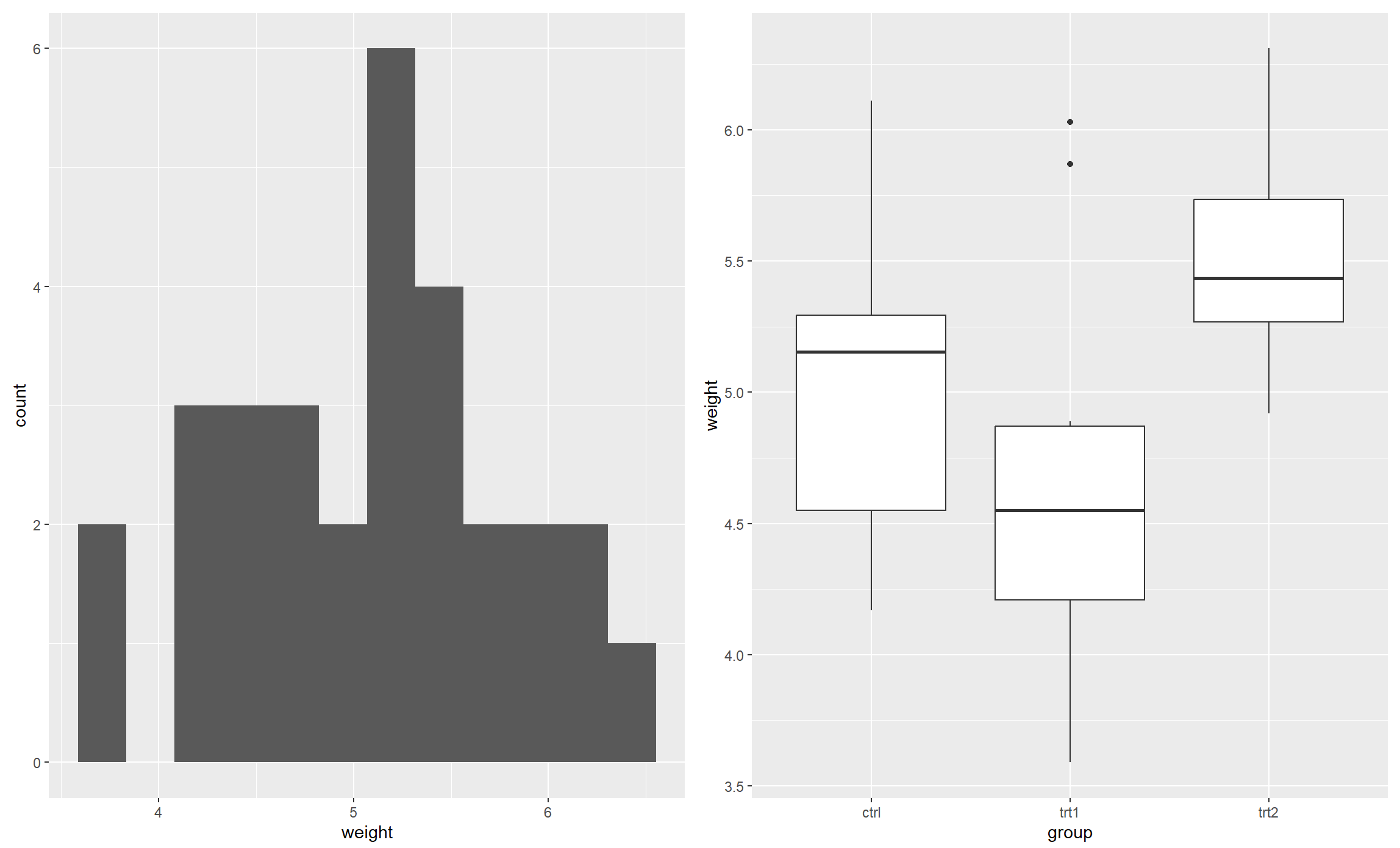
library(patchwork)
library(ggplot2)

plot1 <- ggplot(PlantGrowth, aes(x = weight)) +
  geom_histogram(bins = 12)

plot2 <- ggplot(PlantGrowth, aes(x = group, y = weight, group = group)) +
  geom_boxplot()

plot1 + plot2
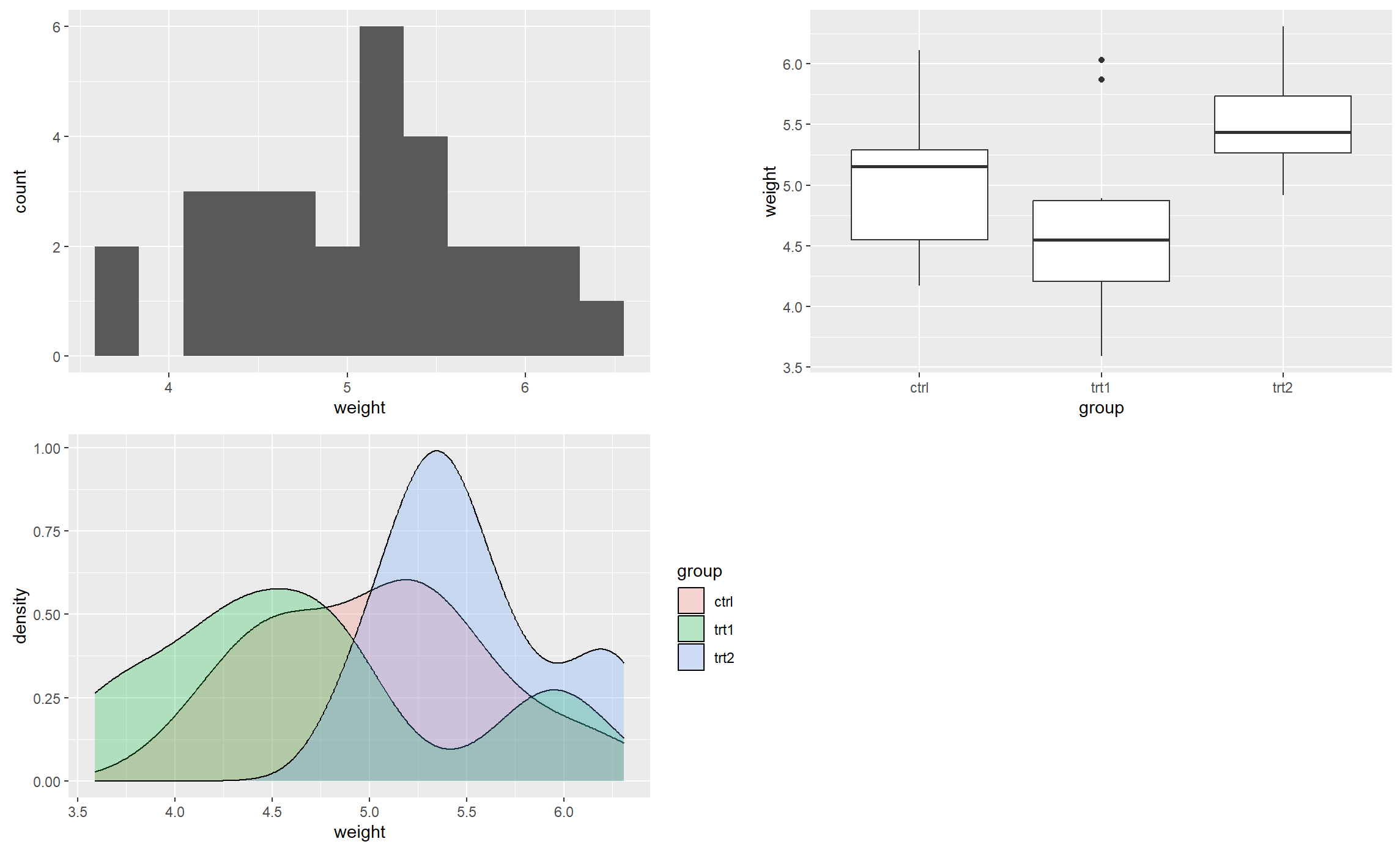
library(patchwork)
library(ggplot2)
plot1 <- ggplot(PlantGrowth, aes(x = weight)) +
  geom_histogram(bins = 12)

plot2 <- ggplot(PlantGrowth, aes(x = group, y = weight, group = group)) +
  geom_boxplot()

plot3 <- ggplot(PlantGrowth, aes(x = weight, fill = group)) +
  geom_density(alpha = 0.25)

plot1 + plot2 + plot3 +
  plot_layout(ncol = 2)
library(patchwork)
library(ggplot2)
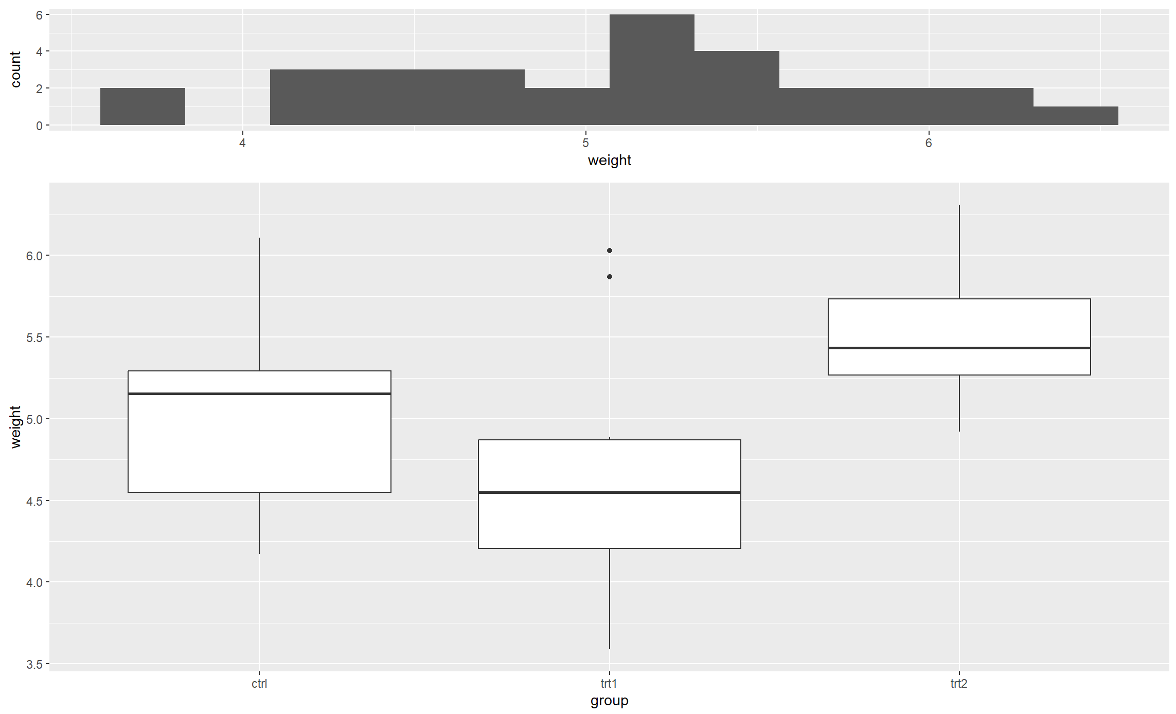
plot1 <- ggplot(PlantGrowth, aes(x = weight)) +
geom_histogram(bins = 12)
plot2 <- ggplot(PlantGrowth, aes(x = group, y = weight, group = group)) +
geom_boxplot()
plot3 <- ggplot(PlantGrowth, aes(x = weight, fill = group)) +
geom_density(alpha = 0.25)
plot1 + plot2 +
plot_layout(ncol = 1, heights = c(1, 4))
library(patchwork)
library(ggplot2)
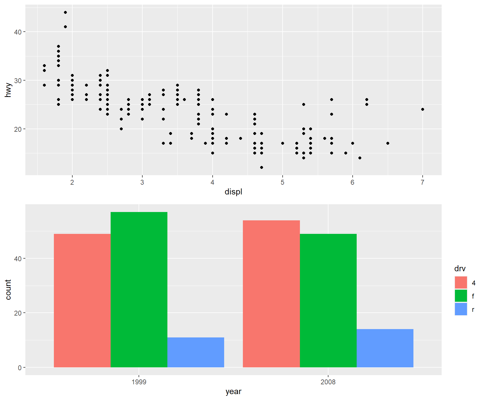
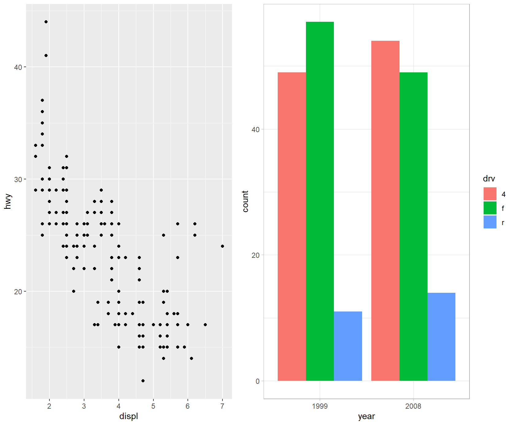
p1 <- ggplot(mpg) +
geom_point(aes(x = displ, y = hwy))
p2 <- ggplot(mpg) +
geom_bar(aes(x = as.character(year), fill = drv), position = "dodge") +
labs(x = "year")
p1 / p2
library(patchwork)
library(ggplot2)
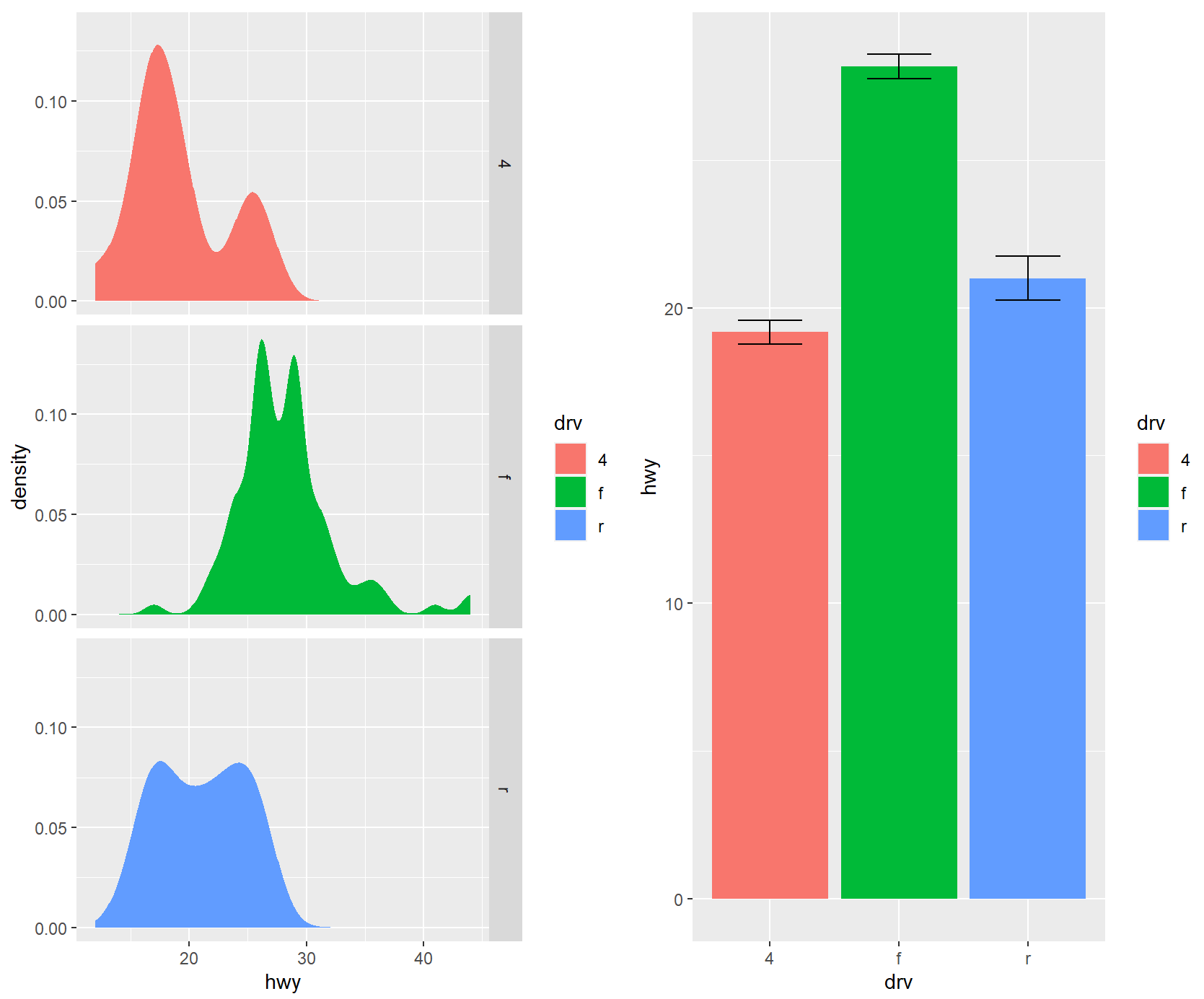
p3 <- ggplot(mpg) +
geom_density(aes(x = hwy, fill = drv), colour = NA) +
facet_grid(rows = vars(drv))
p4 <- ggplot(mpg) +
stat_summary(aes(x = drv, y = hwy, fill = drv), geom = "col", fun.data = mean_se) +
stat_summary(aes(x = drv, y = hwy), geom = "errorbar", fun.data = mean_se, width = 0.5)
p3 | p4
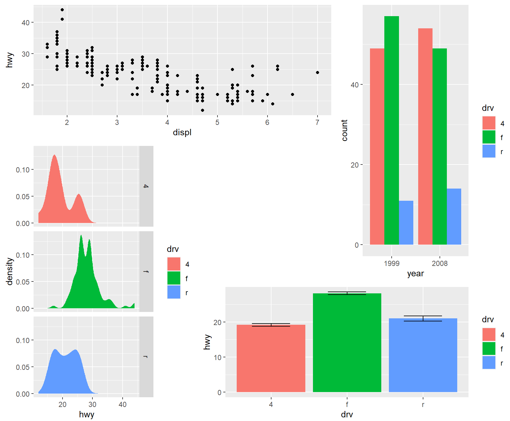
library(patchwork)
library(ggplot2)
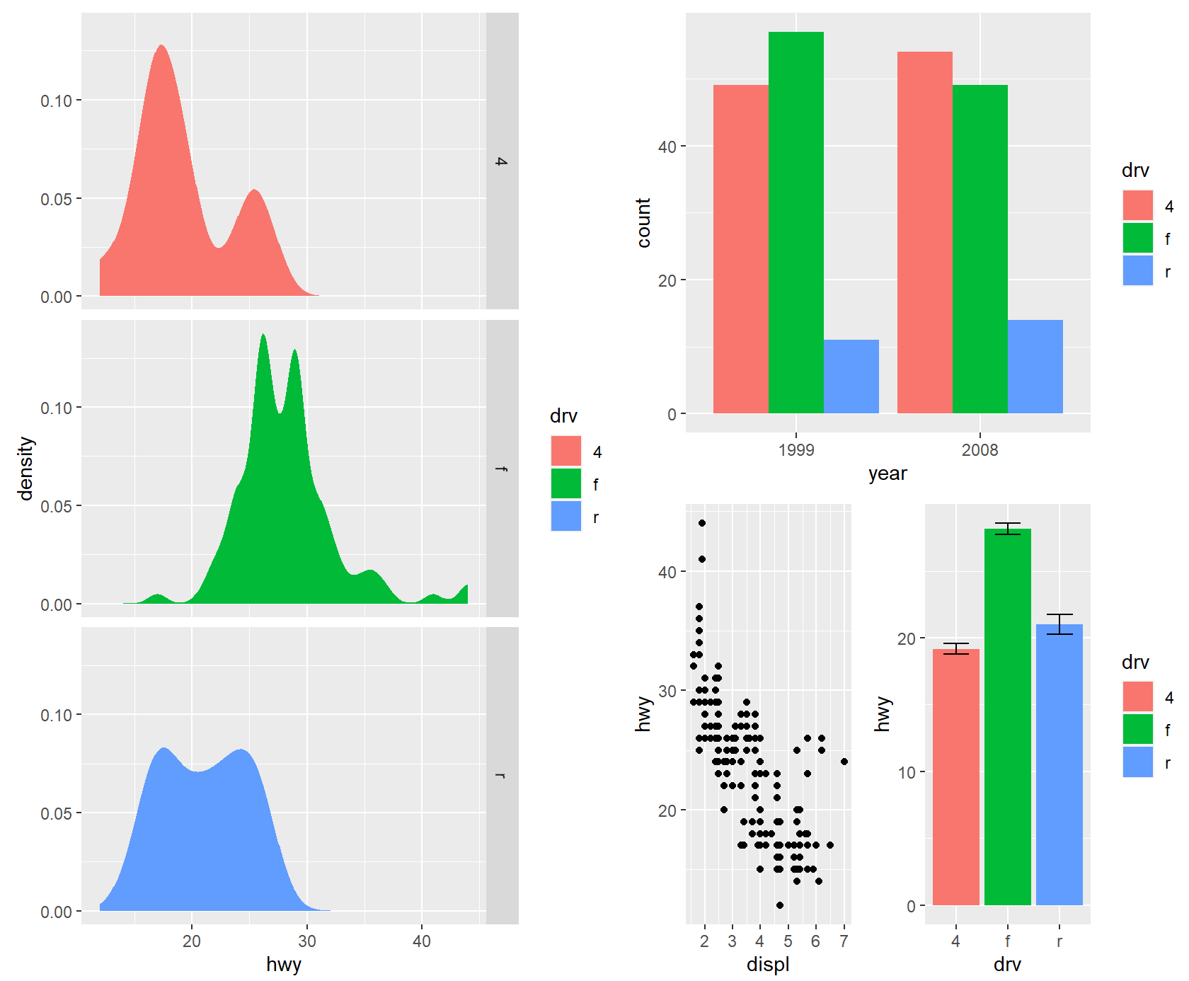
p1 <- ggplot(mpg) +
geom_point(aes(x = displ, y = hwy))
p2 <- ggplot(mpg) +
geom_bar(aes(x = as.character(year), fill = drv), position = "dodge") +
labs(x = "year")
p3 <- ggplot(mpg) +
geom_density(aes(x = hwy, fill = drv), colour = NA) +
facet_grid(rows = vars(drv))
p4 <- ggplot(mpg) +
stat_summary(aes(x = drv, y = hwy, fill = drv), geom = "col", fun.data = mean_se) +
stat_summary(aes(x = drv, y = hwy), geom = "errorbar", fun.data = mean_se, width = 0.5)
p3 | (p2 / (p1 | p4))
library(patchwork)
library(ggplot2)

p1 <- ggplot(mpg) +
  geom_point(aes(x = displ, y = hwy))

p2 <- ggplot(mpg) +
  geom_bar(aes(x = as.character(year), fill = drv), position = "dodge") +
  labs(x = "year")

p3 <- ggplot(mpg) +
  geom_density(aes(x = hwy, fill = drv), colour = NA) +
  facet_grid(rows = vars(drv))

p4 <- ggplot(mpg) +
  stat_summary(aes(x = drv, y = hwy, fill = drv), geom = "col", fun.data = mean_se) +
  stat_summary(aes(x = drv, y = hwy), geom = "errorbar", fun.data = mean_se, width = 0.5)

layout <- "
AAB
C#B
CDD
"

p1 + p2 + p3 + p4 + plot_layout(design = layout)
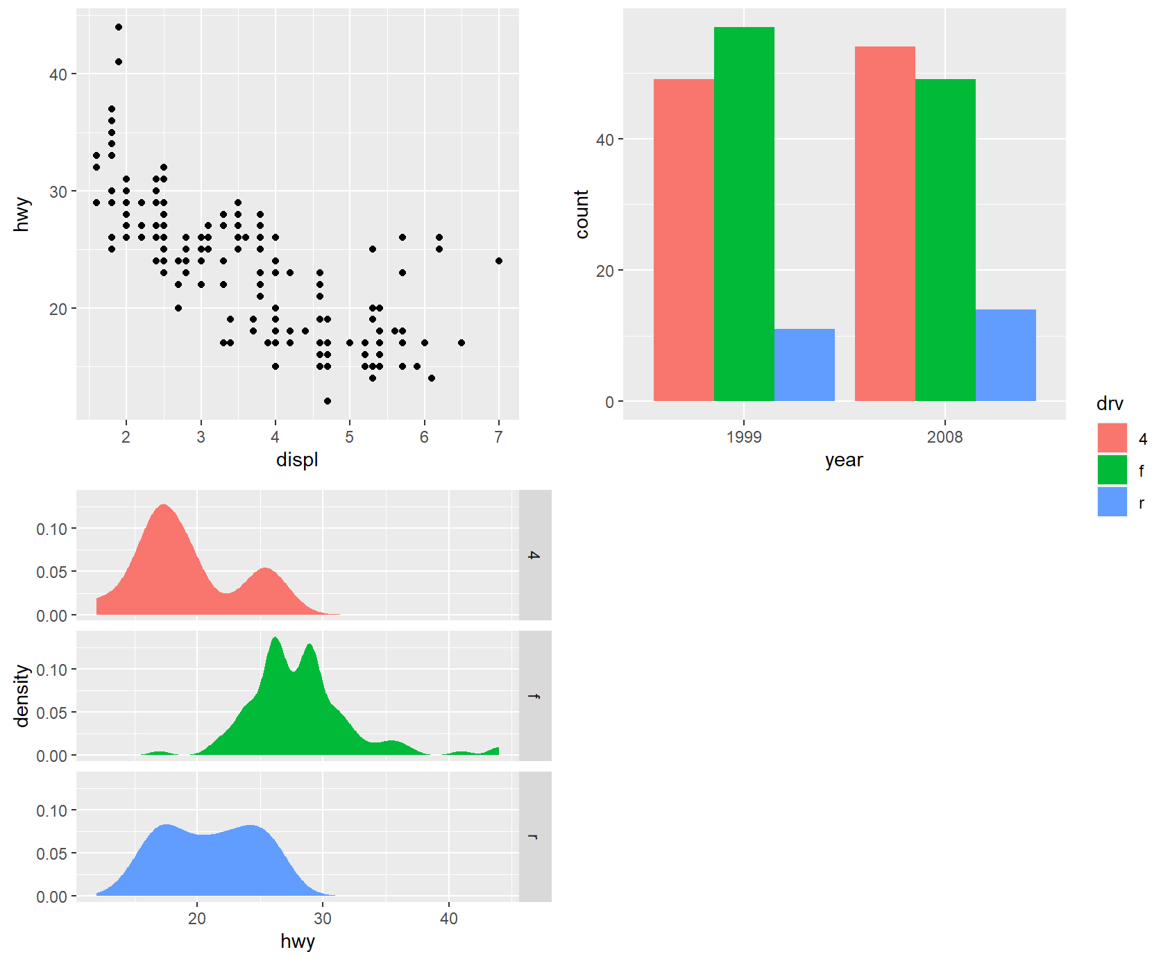
library(patchwork)
library(ggplot2)

p1 <- ggplot(mpg) +
  geom_point(aes(x = displ, y = hwy))

p2 <- ggplot(mpg) +
  geom_bar(aes(x = as.character(year), fill = drv), position = "dodge") +
  labs(x = "year")

p3 <- ggplot(mpg) +
  geom_density(aes(x = hwy, fill = drv), colour = NA) +
  facet_grid(rows = vars(drv))

p1 + p2 + p3 + plot_layout(ncol = 2, guides = "collect")
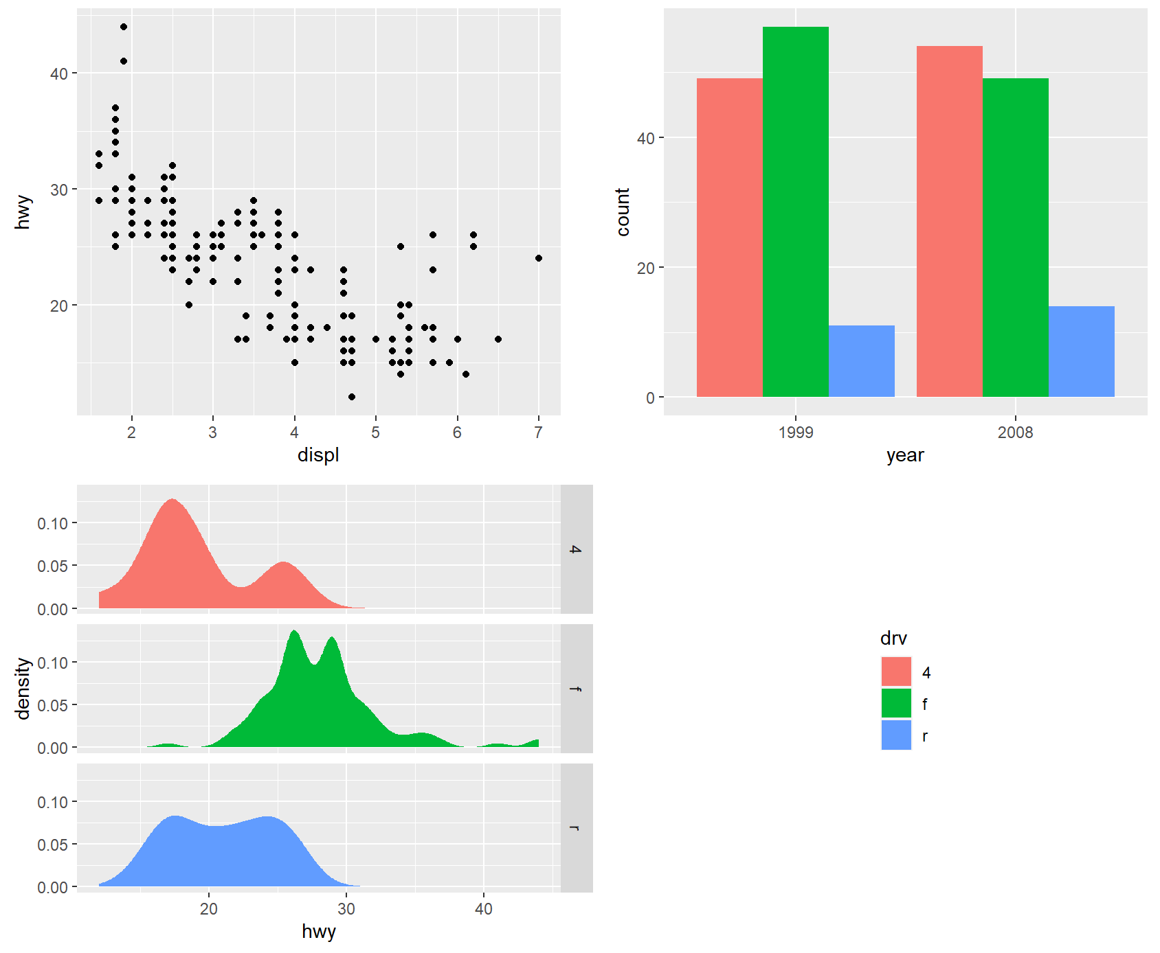
library(patchwork)
library(ggplot2)

p1 <- ggplot(mpg) +
  geom_point(aes(x = displ, y = hwy))

p2 <- ggplot(mpg) +
  geom_bar(aes(x = as.character(year), fill = drv), position = "dodge") +
  labs(x = "year")

p3 <- ggplot(mpg) +
  geom_density(aes(x = hwy, fill = drv), colour = NA) +
  facet_grid(rows = vars(drv))

p1 + p2 + p3 + guide_area() + plot_layout(ncol = 2, guides = "collect")
library(patchwork)
library(ggplot2)

p1 <- ggplot(mpg) +
  geom_point(aes(x = displ, y = hwy))

p2 <- ggplot(mpg) +
  geom_bar(aes(x = as.character(year), fill = drv), position = "dodge") +
  labs(x = "year")

p12 <- p1 + p2
p12[[2]] <- p12[[2]] + theme_light()
p12
library(patchwork)
library(ggplot2)

p1 <- ggplot(mpg) +
  geom_point(aes(x = displ, y = hwy))

p4 <- ggplot(mpg) +
  stat_summary(aes(x = drv, y = hwy, fill = drv), geom = "col", fun.data = mean_se) +
  stat_summary(aes(x = drv, y = hwy), geom = "errorbar", fun.data = mean_se, width = 0.5)

p1 + p4 & theme_minimal()
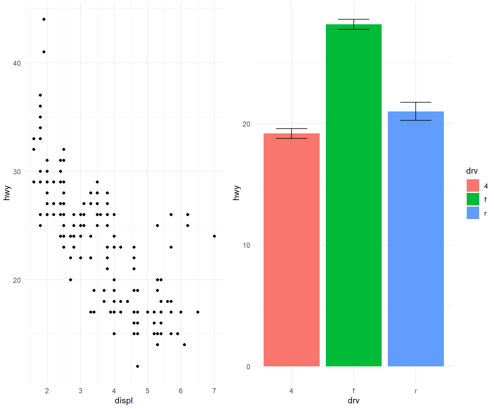
library(patchwork)
library(ggplot2)

p1 <- ggplot(mpg) +
  geom_point(aes(x = displ, y = hwy))

p4 <- ggplot(mpg) +
  stat_summary(aes(x = drv, y = hwy, fill = drv), geom = "col", fun.data = mean_se) +
  stat_summary(aes(x = drv, y = hwy), geom = "errorbar", fun.data = mean_se, width = 0.5)

p1 + p4 & scale_y_continuous(limits = c(0, 45))
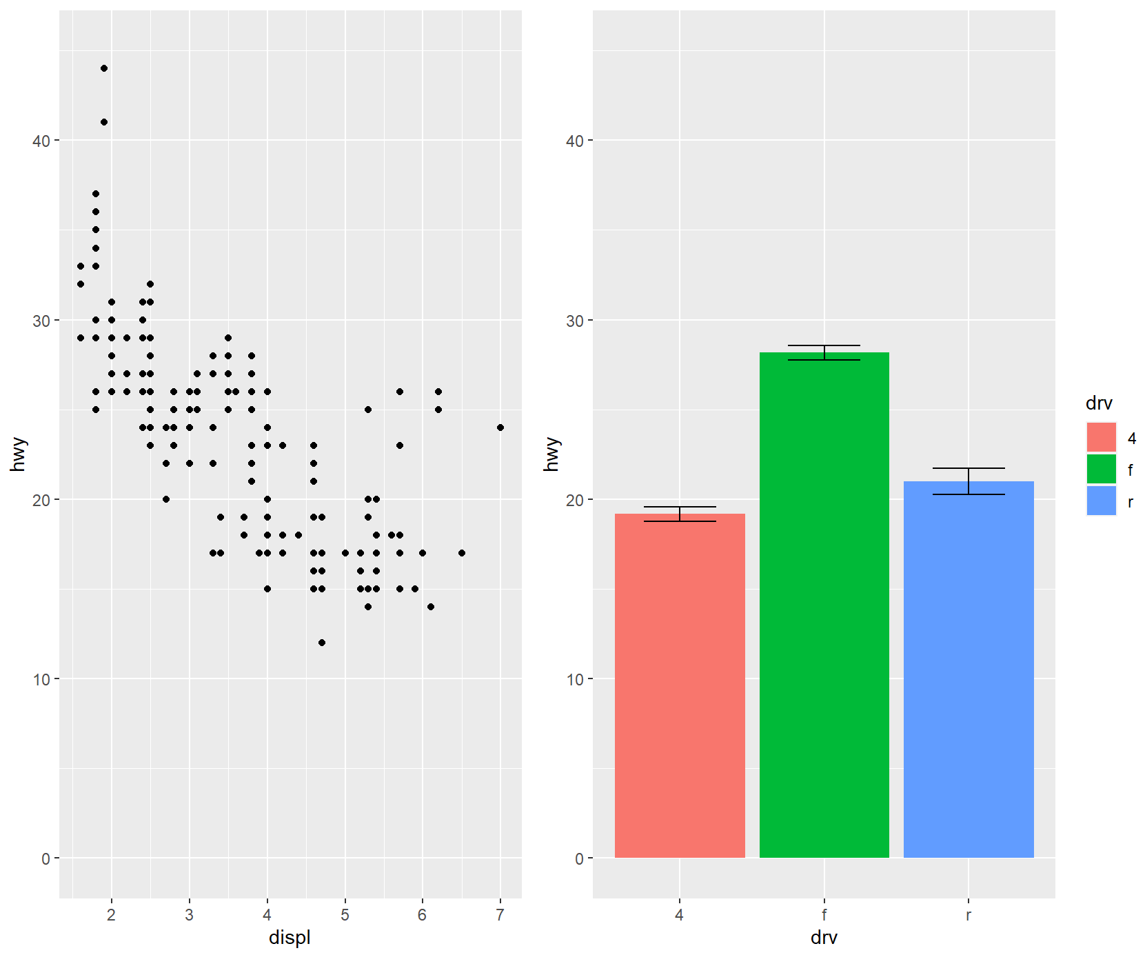
library(patchwork)
library(ggplot2)
p3 <- ggplot(mpg) +
geom_density(aes(x = hwy, fill = drv), colour = NA) +
facet_grid(rows = vars(drv))
p4 <- ggplot(mpg) +
stat_summary(aes(x = drv, y = hwy, fill = drv), geom = "col", fun.data = mean_se) +
stat_summary(aes(x = drv, y = hwy), geom = "errorbar", fun.data = mean_se, width = 0.5)
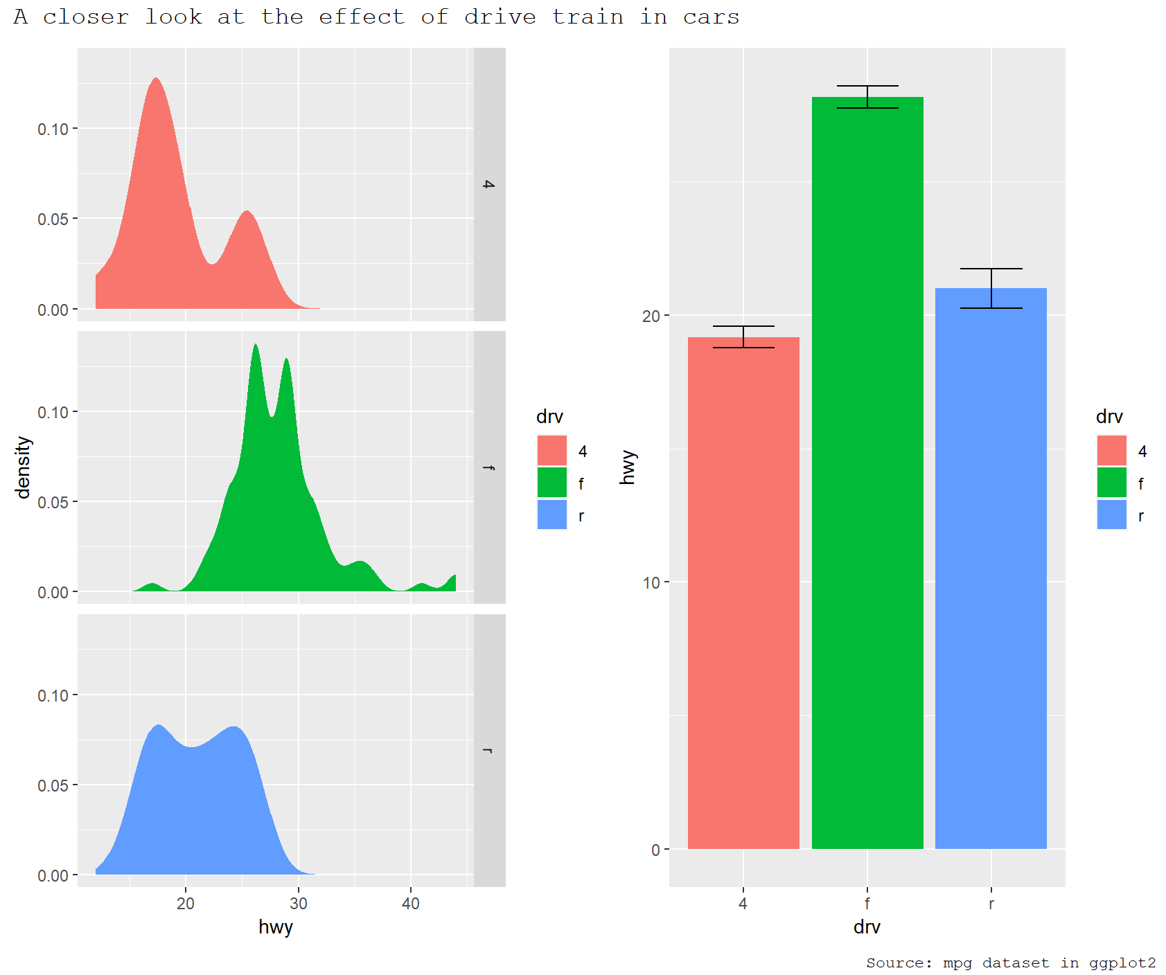
p34 <- p3 + p4 + plot_annotation(
title = "A closer look at the effect of drive train in cars",
caption = "Source: mpg dataset in ggplot2"
)
p34

library(patchwork)
library(ggplot2)
p3 <- ggplot(mpg) +
geom_density(aes(x = hwy, fill = drv), colour = NA) +
facet_grid(rows = vars(drv))
p4 <- ggplot(mpg) +
stat_summary(aes(x = drv, y = hwy, fill = drv), geom = "col", fun.data = mean_se) +
stat_summary(aes(x = drv, y = hwy), geom = "errorbar", fun.data = mean_se, width = 0.5)
p34 <- p3 + p4 + plot_annotation(
title = "A closer look at the effect of drive train in cars",
caption = "Source: mpg dataset in ggplot2"
)
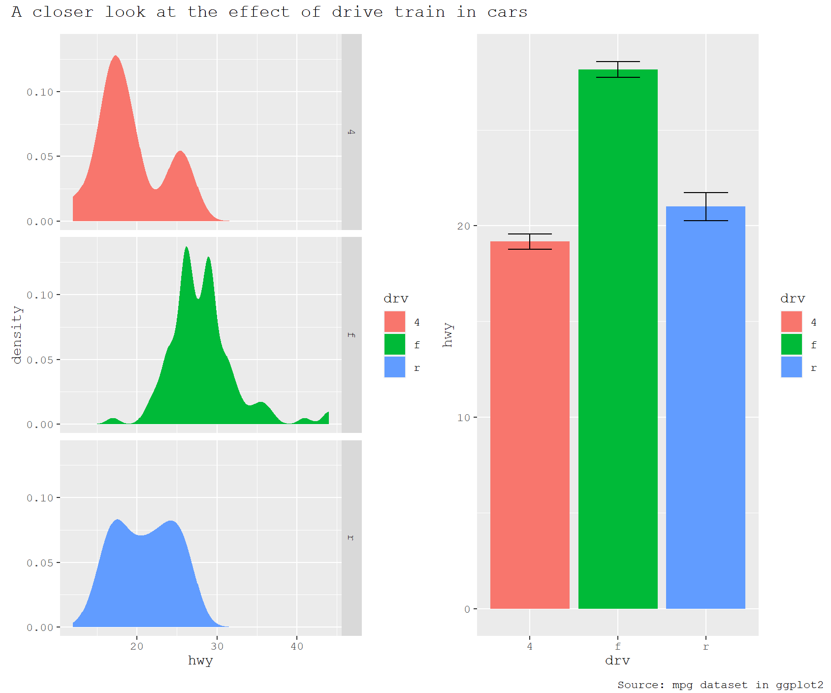
p34 + plot_annotation(theme = theme_gray(base_family = "mono"))
library(patchwork)
library(ggplot2)

p3 <- ggplot(mpg) +
  geom_density(aes(x = hwy, fill = drv), colour = NA) +
  facet_grid(rows = vars(drv))

p4 <- ggplot(mpg) +
  stat_summary(aes(x = drv, y = hwy, fill = drv), geom = "col", fun.data = mean_se) +
  stat_summary(aes(x = drv, y = hwy), geom = "errorbar", fun.data = mean_se, width = 0.5)

p34 <- p3 + p4 + plot_annotation(
  title = "A closer look at the effect of drive train in cars",
  caption = "Source: mpg dataset in ggplot2"
)
p34 & theme_gray(base_family = "mono")
library(patchwork)
library(ggplot2)
p1 <- ggplot(mpg) +
geom_point(aes(x = displ, y = hwy))
p2 <- ggplot(mpg) +
geom_bar(aes(x = as.character(year), fill = drv), position = "dodge") +
labs(x = "year")
p3 <- ggplot(mpg) +
geom_density(aes(x = hwy, fill = drv), colour = NA) +
facet_grid(rows = vars(drv))
p123 <- p1 | (p2 / p3)
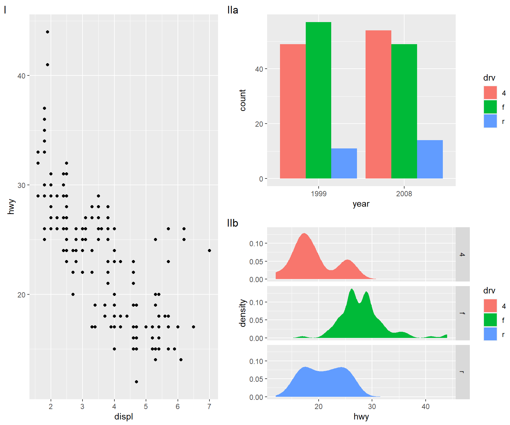
p123 + plot_annotation(tag_levels = "I") # Uppercase roman numerics

library(patchwork)
library(ggplot2)

p1 <- ggplot(mpg) +
  geom_point(aes(x = displ, y = hwy))

p2 <- ggplot(mpg) +
  geom_bar(aes(x = as.character(year), fill = drv), position = "dodge") +
  labs(x = "year")

p3 <- ggplot(mpg) +
  geom_density(aes(x = hwy, fill = drv), colour = NA) +
  facet_grid(rows = vars(drv))

p123 <- p1 | (p2 / p3)
p123[[2]] <- p123[[2]] + plot_layout(tag_level = "new")
p123 + plot_annotation(tag_levels = c("I", "a"))
library(patchwork)
library(ggplot2)
p1 <- ggplot(mpg) +
geom_point(aes(x = displ, y = hwy))
p2 <- ggplot(mpg) +
geom_bar(aes(x = as.character(year), fill = drv), position = "dodge") +
labs(x = "year")
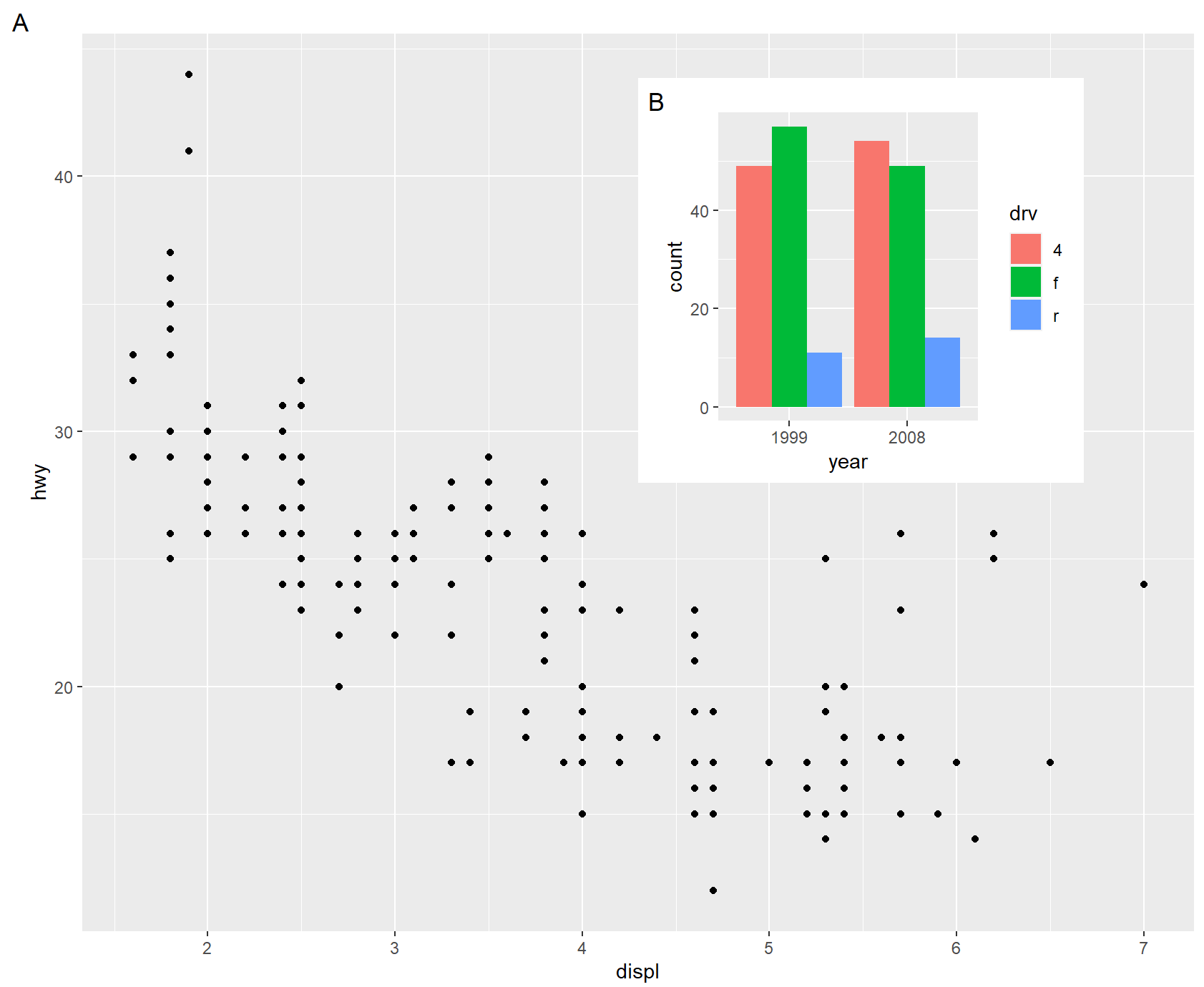
p1 + inset_element(p2, left = 0.5, bottom = 0.4, right = 0.9, top = 0.95)
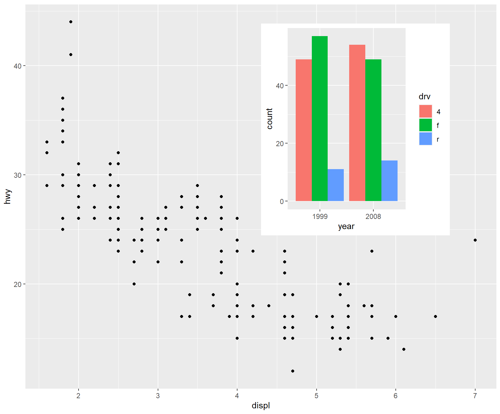
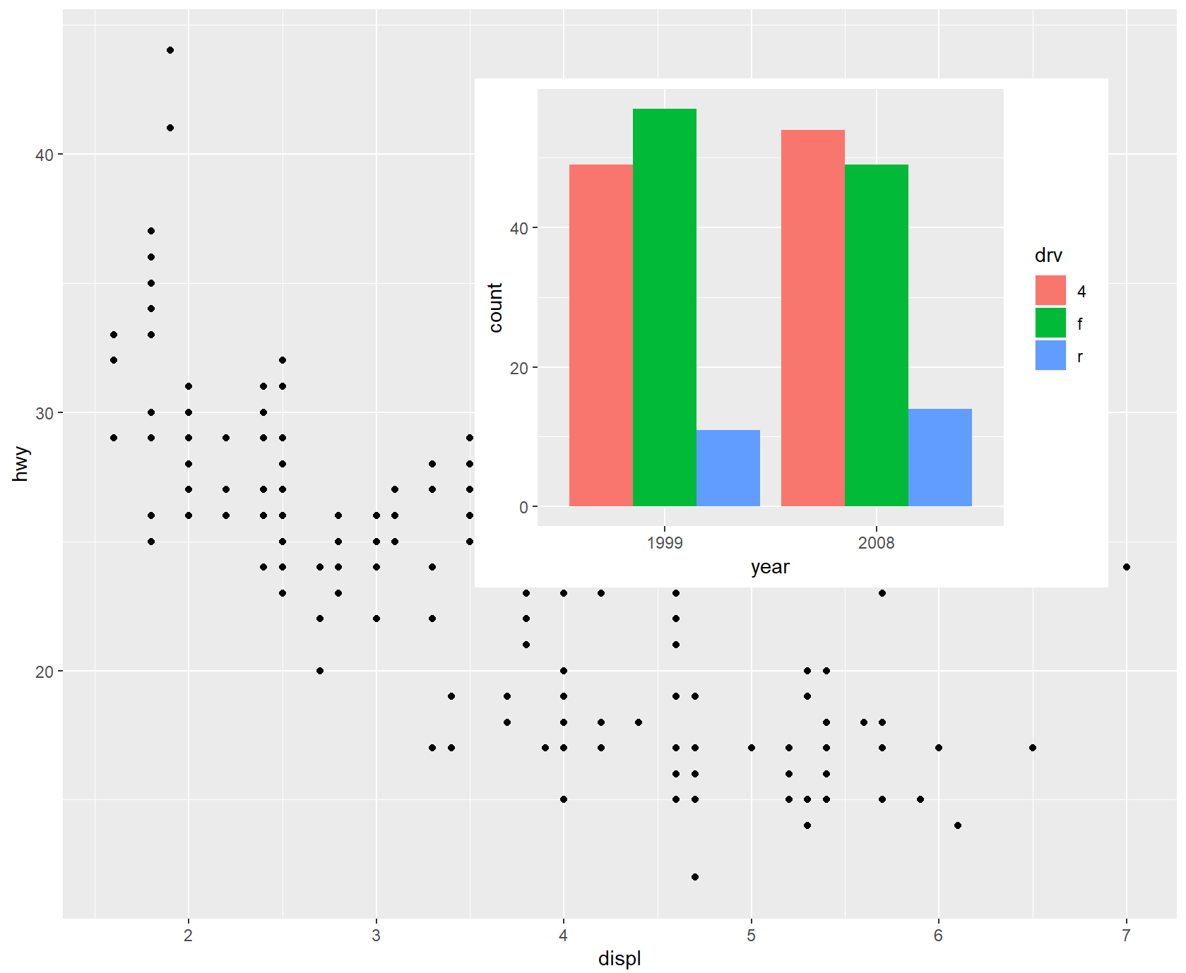
The position is specified by given the left, right, top, and bottom location of the inset. The default is to use npc units which goes from 0 to 1 in the given area, but any grid::unit() can be used by giving them explicitly. The location is by default set to the panel area, but this can be changed with the align_to argument. Combining all this we can place an inset exactly 15 mm from the top right corner like this:
library(patchwork)
library(ggplot2)

p1 <- ggplot(mpg) +
  geom_point(aes(x = displ, y = hwy))

p2 <- ggplot(mpg) +
  geom_bar(aes(x = as.character(year), fill = drv), position = "dodge") +
  labs(x = "year")

p1 +
  inset_element(
    p2,
    left = 0.4,
    bottom = 0.4,
    right = unit(1, "npc") - unit(15, "mm"),
    top = unit(1, "npc") - unit(15, "mm"),
    align_to = "full"
  )
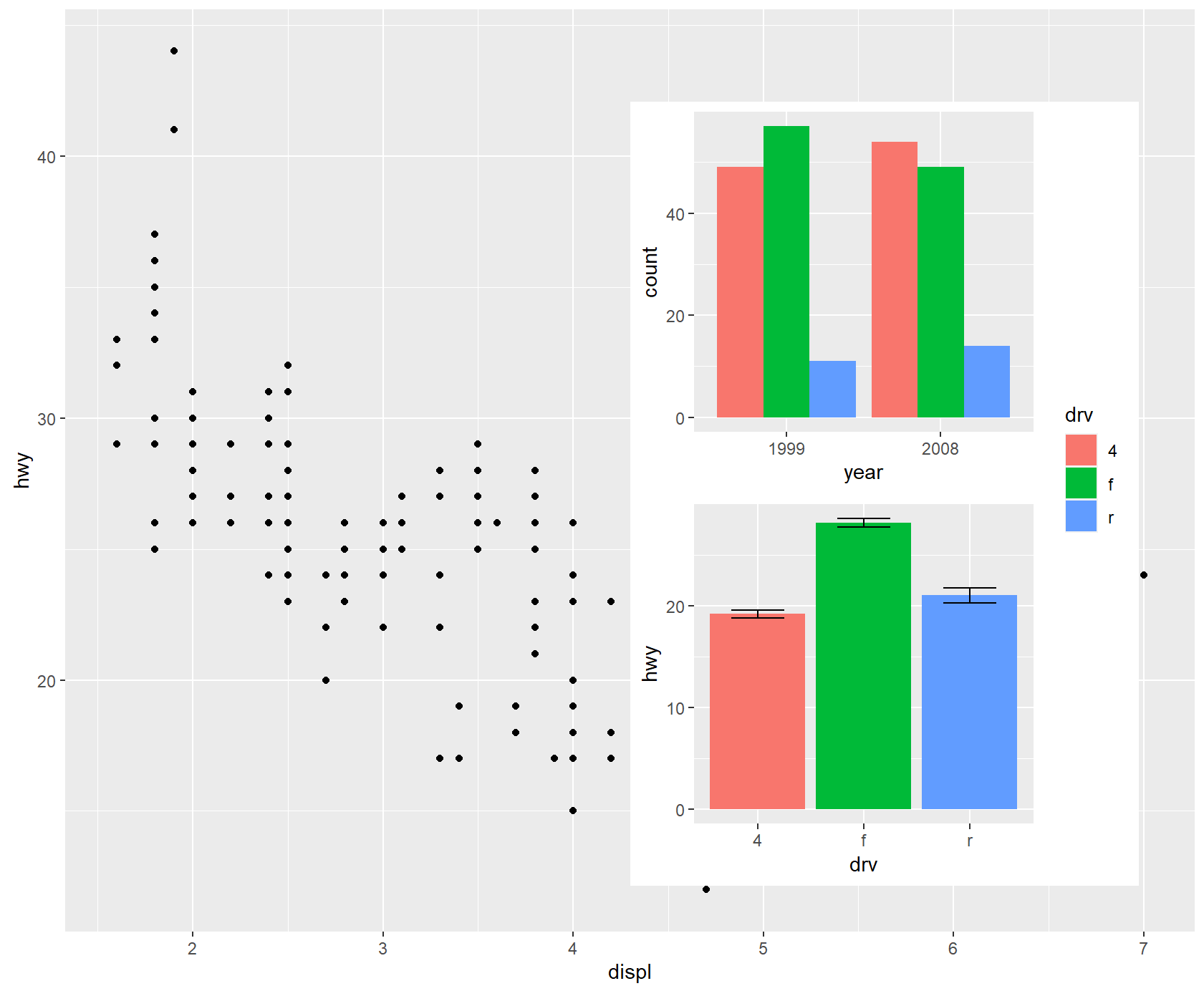
library(patchwork)
library(ggplot2)

p1 <- ggplot(mpg) +
  geom_point(aes(x = displ, y = hwy))

p2 <- ggplot(mpg) +
  geom_bar(aes(x = as.character(year), fill = drv), position = "dodge") +
  labs(x = "year")

p4 <- ggplot(mpg) +
  stat_summary(aes(x = drv, y = hwy, fill = drv), geom = "col", fun.data = mean_se) +
  stat_summary(aes(x = drv, y = hwy), geom = "errorbar", fun.data = mean_se, width = 0.5)

p24 <- p2 / p4 + plot_layout(guides = "collect")
p1 + inset_element(p24, left = 0.5, bottom = 0.05, right = 0.95, top = 0.9)
library(patchwork)
library(ggplot2)

p1 <- ggplot(mpg) +
  geom_point(aes(x = displ, y = hwy))

p2 <- ggplot(mpg) +
  geom_bar(aes(x = as.character(year), fill = drv), position = "dodge") +
  labs(x = "year")

p12 <- p1 + inset_element(p2, left = 0.5, bottom = 0.5, right = 0.9, top = 0.95)
p12 & theme_bw()

library(patchwork)
library(ggplot2)

p1 <- ggplot(mpg) +
  geom_point(aes(x = displ, y = hwy))

p2 <- ggplot(mpg) +
  geom_bar(aes(x = as.character(year), fill = drv), position = "dodge") +
  labs(x = "year")

p12 <- p1 + inset_element(p2, left = 0.5, bottom = 0.5, right = 0.9, top = 0.95)
p12 + plot_annotation(tag_levels = "A")
更多细节可参考:https://github.com/thomasp85/patchwork
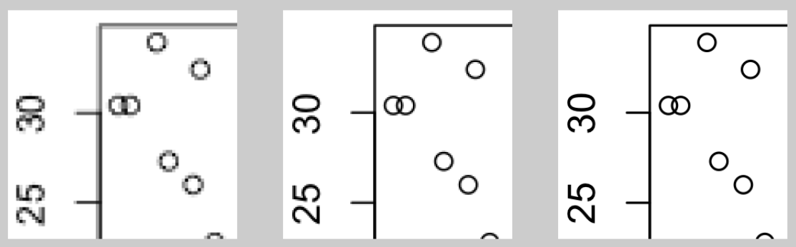
useDingbats参数
Adobe Illustrator修图时,可能会出现pdf中的圆形被绘制为字体字符,通过设定useDingbats = FALSE可避免该情况。
pdf("myplot.pdf", width = 4, height = 4, useDingbats = FALSE)

# 或者
ggsave("myplot.pdf", width = 4, height = 4, useDingbats = FALSE)
参考资料
- R语言实战(第三版)
- ggplot2:数据分析与图形艺术(第2版)
- R语言医学数据分析实战
- https://ggplot2-book.org/arranging-plots
- https://r-graphics.org/


 6558
6558


 被折叠的 条评论
为什么被折叠?
被折叠的 条评论
为什么被折叠?
 到【灌水乐园】发言


