


1. 复现论文简介
该论文主要研究了离散时间确定性非线性系统的一种新型策略迭代型确定性Q学习算法。该算法的推导和与之前的Q学习算法的区别进行了讨论,对算法的收敛性和稳定性等性质进行了分析,采用神经网络实现了该算法,并通过仿真结果证明了其有效性。
参考文献:
[1] Wei, Qinglai, Ruizhuo Song, Benkai Li, Xiaofeng Lin. “A novel policy iteration-based deterministic Q-learning for discrete-time nonlinear systems.” Self-Learning Optimal Control of Nonlinear Systems: Adaptive Dynamic Programming Approach (2018): 85-109.
2. 具体算法实现

算法总结:
- 初始化神经网络的结构和权重;
- 随机选择一定数量的训练数据;
- 使用策略迭代型确定性Q学习算法对神经网络进行训练,迭代更新权重;
- 重复步骤3直到神经网络的训练误差小于设定阈值;
- 根据训练好的神经网络得到最优控制策略。
3. 系统模型及仿真结果
原论文主要在线性系统和扭摆非线性系统进行仿真验证,发现提出的策略迭代型确定性Q学习算法在离散时间的非线性系统取得了不错的效果。
在本次复现中,分别采用扭摆非线性系统算例、质量弹簧阻尼系统以及非线性数值算例进行仿真,通过在三个模型的仿真结果,的确说明了该算法的有效性。复现论文不易,有需要源代码的同学,请私信联系。
文献出处:
[1] Liu D , Wei Q . Policy Iteration Adaptive Dynamic Programming Algorithm for Discrete-Time Nonlinear Systems[J]. IEEE Trans Neural Netw Learn Syst, 2014, 25(3):621-634.
[2] Mu C , Wang D , He H . Novel iterative neural dynamic programming for data-based approximate optimal control design[J]. Automatica, 2017, 81:240-252.
Dynamic:
{
d
θ
d
t
=
ω
J
d
ω
d
t
=
u
−
M
g
l
sin
θ
−
f
d
d
θ
d
t
\left\{\begin{array}{l} \frac{d \theta}{d t}=\omega \\ J \frac{d \omega}{d t}=u-M g l \sin \theta-f_{d} \frac{d \theta}{d t} \end{array}\right.
{dtdθ=ωJdtdω=u−Mglsinθ−fddtdθ
where
M
=
1
/
3
k
g
M=1 / 3 \mathrm{kg}
M=1/3kg and
l
=
2
/
3
m
l=2 / 3 \mathrm{m}
l=2/3m are the mass and length of the pendulum bar, respectively. The system states are the current angle
θ
\theta
θ and the angular velocity
ω
.
\omega .
ω. Let
J
=
4
/
3
M
l
2
J=4 / 3 M l^{2}
J=4/3Ml2 and
f
d
=
0.2
f_{d}=0.2
fd=0.2 be the rotary inertia and frictional factor, respectively. Let
g
=
9.8
m
/
s
2
g=9.8 \mathrm{m} / \mathrm{s}^{2}
g=9.8m/s2 be the gravity. Discretization of the system function and performance index function using Euler and trapezoidal methods with the sampling interval
Δ
t
=
0.1
s
\Delta t=0.1 \mathrm{s}
Δt=0.1s leads to
[
x
1
(
k
+
1
)
x
2
(
k
+
1
)
]
=
[
0.1
x
2
k
+
x
1
k
−
0.49
×
sin
(
x
1
k
)
−
0.1
×
f
d
×
x
2
k
+
x
2
k
]
+
[
0
0.1
]
u
k
\begin{array}{r} {\left[\begin{array}{c} x_{1(k+1)} \\ x_{2(k+1)} \end{array}\right]=\left[\begin{array}{c} 0.1 x_{2 k}+x_{1 k} \\ -0.49 \times \sin \left(x_{1 k}\right)-0.1 \times f_{d} \times x_{2 k}+x_{2 k} \end{array}\right]} +\left[\begin{array}{c} 0 \\ 0.1 \end{array}\right] u_{k} \end{array}
[x1(k+1)x2(k+1)]=[0.1x2k+x1k−0.49×sin(x1k)−0.1×fd×x2k+x2k]+[00.1]uk
or
x
t
+
1
=
[
x
1
t
+
0.1
x
2
t
0.2
(
−
0.49
sin
(
x
1
t
)
−
0.2
x
2
t
+
x
2
t
)
]
+
[
0
0.02
]
u
t
x_{t+1}=\left[\begin{array}{c} x_{1 t}+0.1 x_{2 t} \\ 0.2\left(-0.49 \sin \left(x_{1 t}\right)-0.2 x_{2 t}+x_{2 t}\right) \end{array}\right]+\left[\begin{array}{c} 0 \\ 0.02 \end{array}\right] u_{t}
xt+1=[x1t+0.1x2t0.2(−0.49sin(x1t)−0.2x2t+x2t)]+[00.02]ut
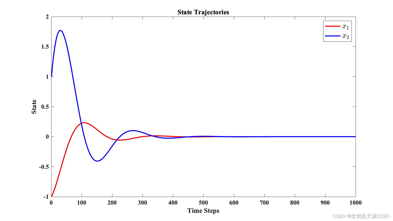
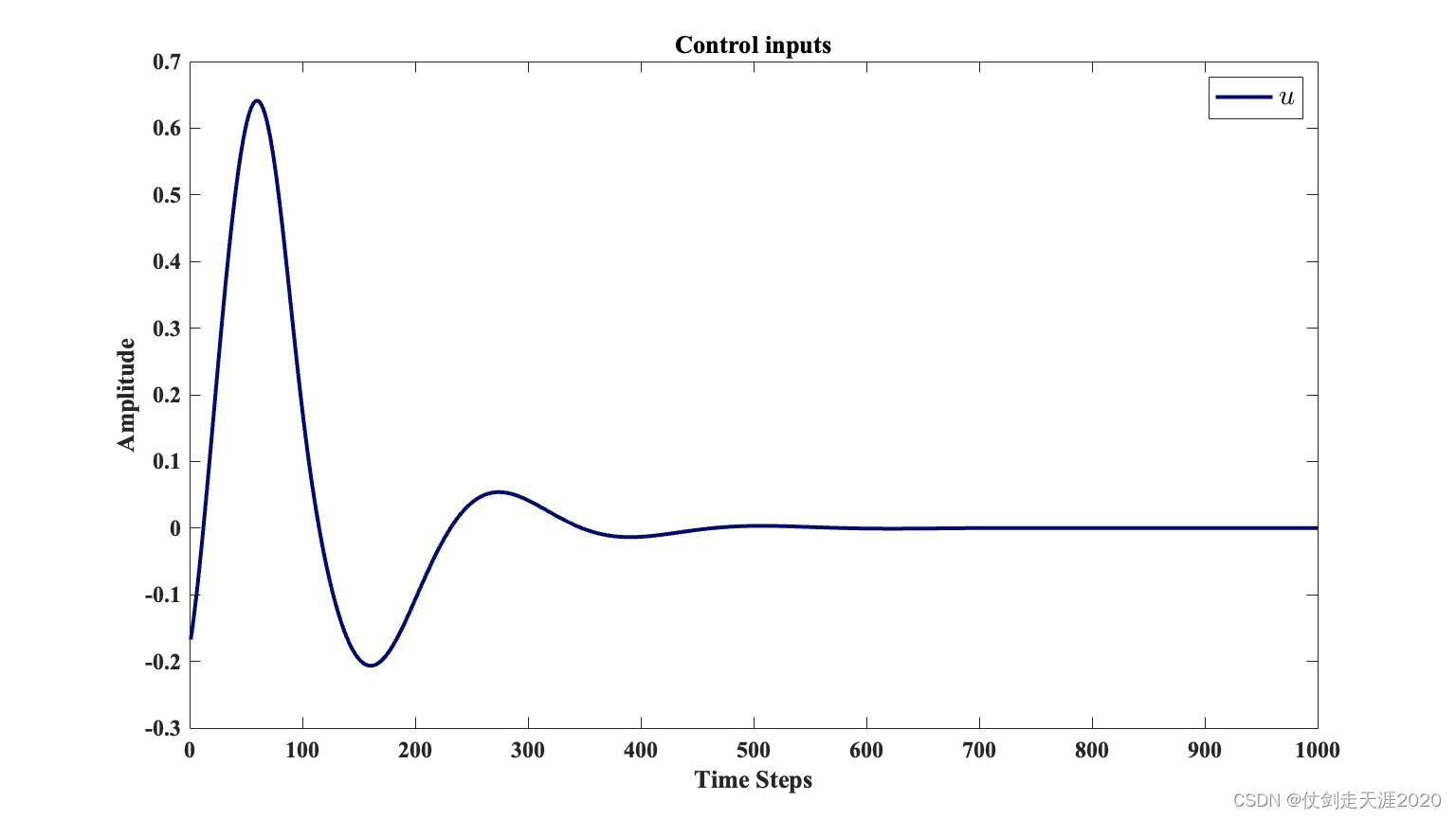
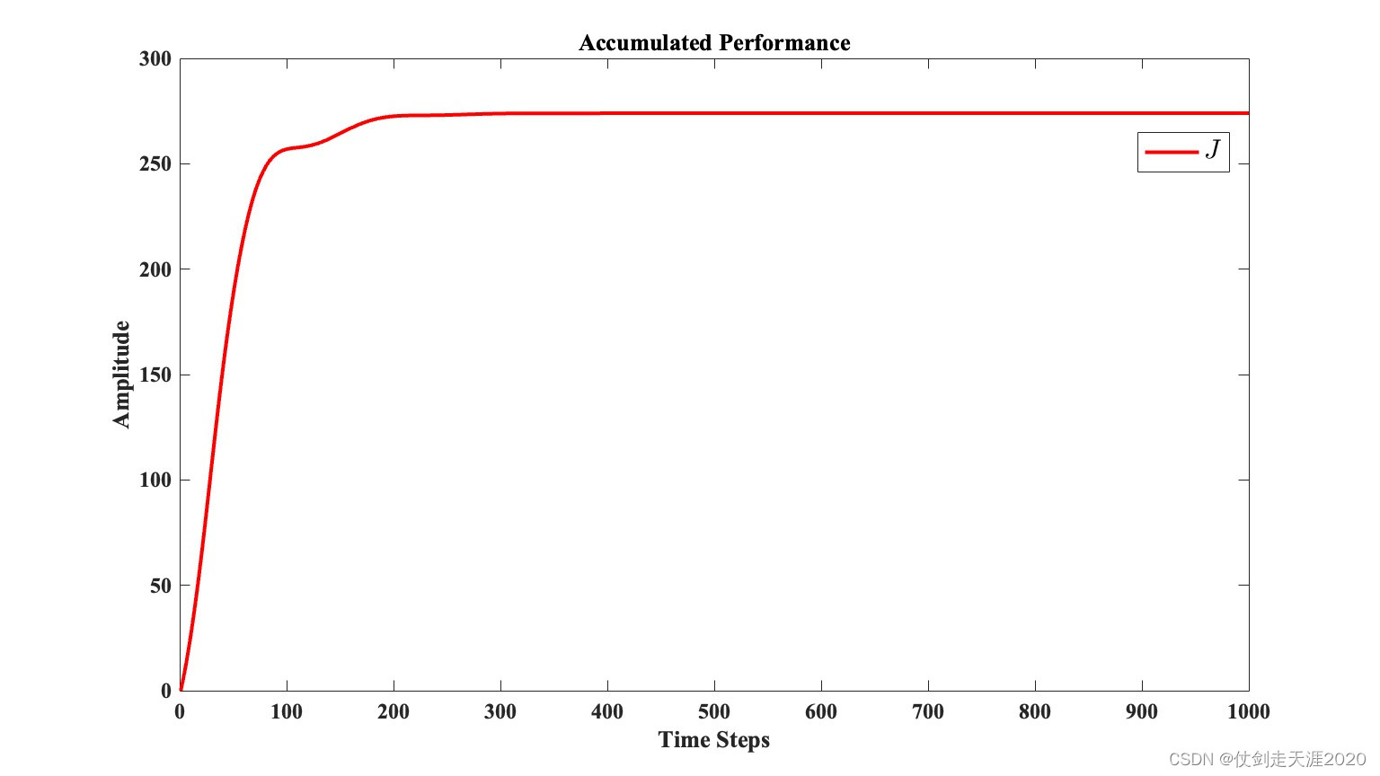
The initial state is
x
0
=
[
1
,
−
1
]
T
x_{0}=[1,-1]^{T}
x0=[1,−1]T.
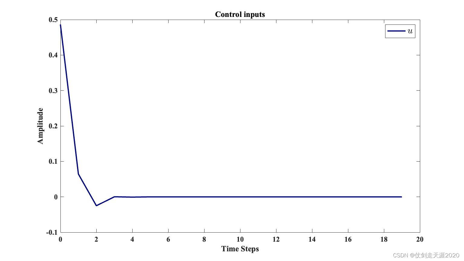
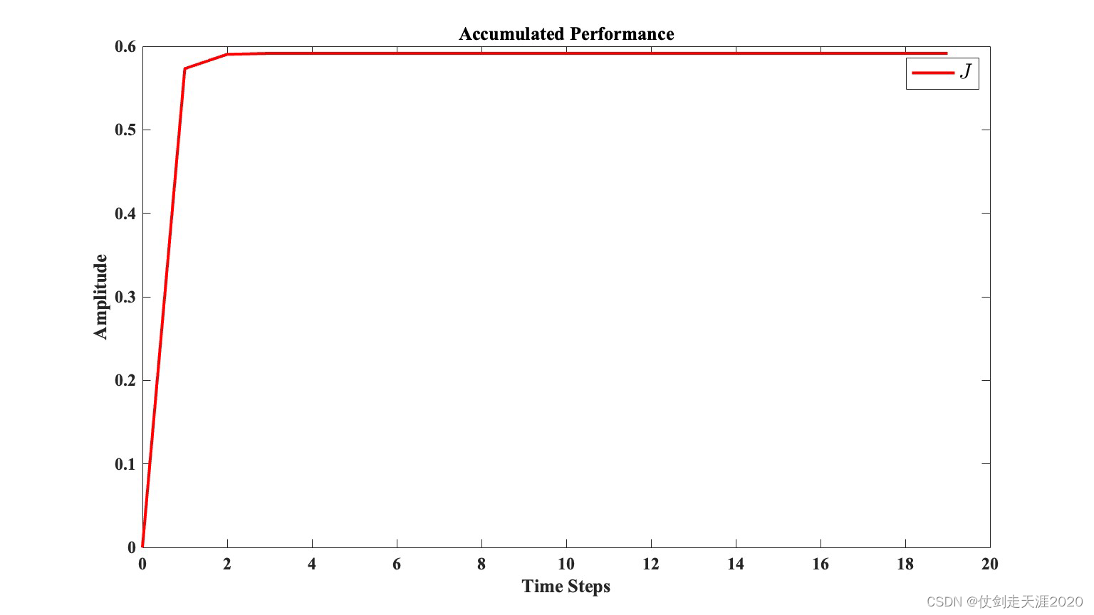
仿真结果:PI_QLearning_case1.m


文献出处:
[1] Winston Alexander Baker. Observer incorporated neoclassical controller design: A discrete perspective[J]. Dissertations & Theses - Gradworks, 2010.
[
x
1
(
k
+
1
)
x
2
(
k
+
1
)
]
=
[
0.0099
x
2
k
+
0.9996
x
1
k
−
0.0887
x
1
k
+
0.97
x
2
k
]
+
[
0
0.0099
]
u
(
k
)
\left[\begin{array}{l} x_{1}(k+1) \\ x_{2}(k+1) \end{array}\right]=\left[\begin{array}{c} 0.0099 x_{2 k}+0.9996 x_{1 k} \\ -0.0887 x_{1 k}+0.97 x_{2 k} \end{array}\right]+\left[\begin{array}{c} 0 \\ 0.0099 \end{array}\right] u(k)
[x1(k+1)x2(k+1)]=[0.0099x2k+0.9996x1k−0.0887x1k+0.97x2k]+[00.0099]u(k)
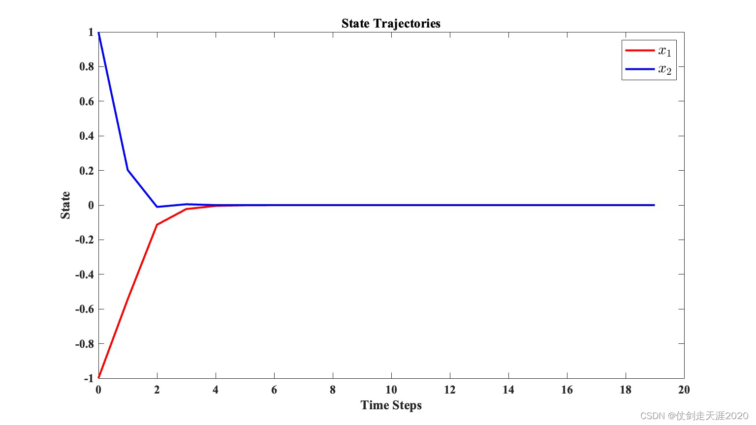
The initial state vector is set as
x
0
=
[
−
1
,
1
]
T
x_{0}=[-1,1]^{T}
x0=[−1,1]T.
仿真结果:PI_QLearning_case2.m
文献出处:
[1] Wang F Y , Jin N , Liu D , et al. Adaptive dynamic programming for finite-horizon optimal control of discrete-time nonlinear systems with ε-error bound.[J]. IEEE Trans Neural Netw, 2011, 22(1):24-36.
[2] Zhang H , Wei Q , Luo Y . A Novel Infinite-Time Optimal Tracking Control Scheme for a Class of Discrete-Time Nonlinear Systems via the Greedy HDP Iteration Algorithm[J]. IEEE Transactions on Systems Man & Cybernetics Part B, 2008, 38(4):937-942.
[3] Liu D , Wei Q . Policy Iteration Adaptive Dynamic Programming Algorithm for Discrete-Time Nonlinear Systems[J]. IEEE Trans Neural Netw Learn Syst, 2014, 25(3):621-634.
We consider the following nonlinear system:
KaTeX parse error: No such environment: align at position 8: \begin{̲a̲l̲i̲g̲n̲}̲ x_{k+1}=f\left…
The system functions are given as
KaTeX parse error: No such environment: align at position 8: \begin{̲a̲l̲i̲g̲n̲}̲ f\left(x_{k}\r…
The initial state is
x
0
=
[
2
,
−
1
]
T
x_{0}=[2,-1]^{T}
x0=[2,−1]T.
仿真结果:PI_QLearning_case3.m


 910
910


 被折叠的 条评论
为什么被折叠?
被折叠的 条评论
为什么被折叠?
 到【灌水乐园】发言


