


目录
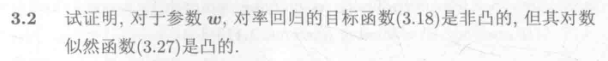
3.1:
解:
首先要明白偏置项b的作用:偏置项在线性回归中起到了调整模型基线、提高拟合能力和简化计算的作用。它使得模型更灵活、更具表达能力,从而能够更好地拟合实际数据分布和反映真实情况。
可以看做是其它变量留下的偏差的线性修正,因此一般情况下是需要考虑偏置项的。但如果对数据集进行了归一化处理,即对目标变量减去均值向量,此时就不需要考虑偏置项了。
3.2:
解:
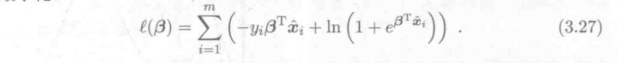
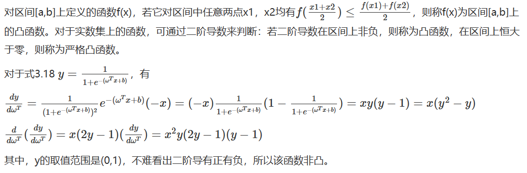
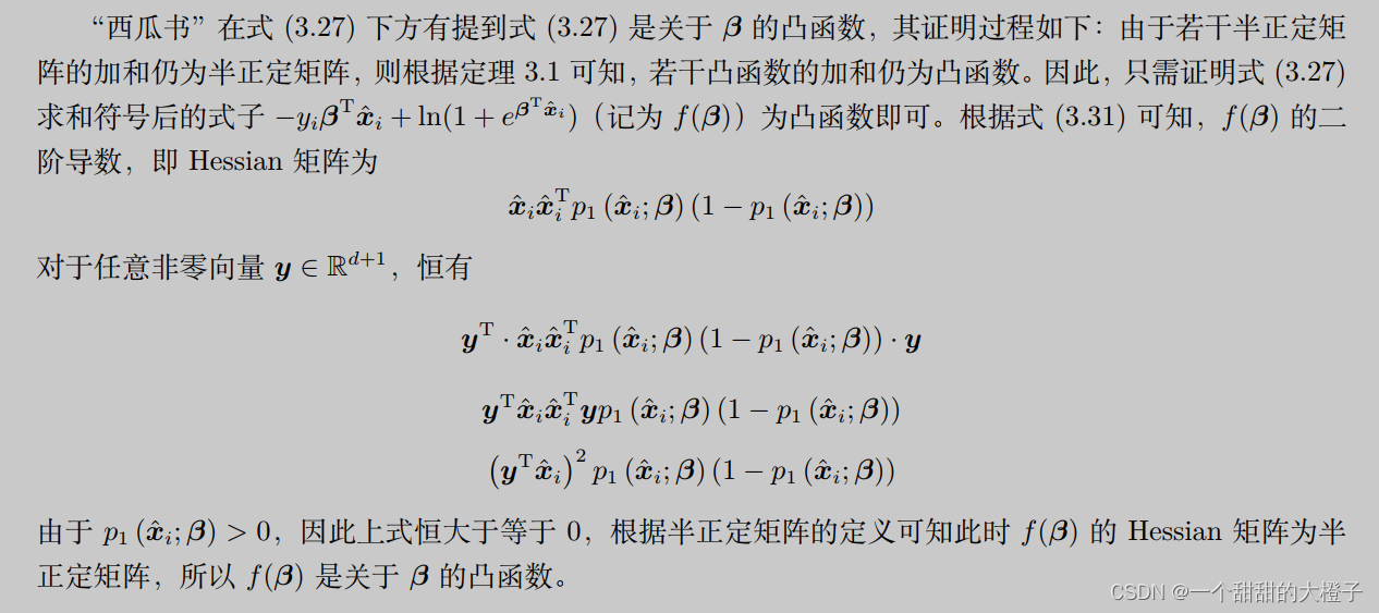
对实数集上的函数,可通过求二阶导数来判别:若二阶导数在区间上非负,则称为凸函数;若二阶导数在区间上恒大于 0,则称为严格凸函数。 对于多元函数,其Hessian matrix为半正定即为凸函数。
3.3:
![]()
解:
"""
与原书不同,原书中一个样本xi 为列向量,本代码中一个样本xi为行向量
尝试了两种优化方法,梯度下降和牛顿法。两者结果基本相同,不过有时因初始化的原因,
会导致牛顿法中海森矩阵为奇异矩阵,np.linalg.inv(hess)会报错。以后有机会再写拟牛顿法吧。
"""
import numpy as np
import pandas as pd
from matplotlib import pyplot as plt
from sklearn import linear_model
def sigmoid(x):
s = 1 / (1 + np.exp(-x))
return s
def J_cost(X, y, beta):
"""
:param X: sample array, shape(n_samples, n_features)
:param y: array-like, shape (n_samples,)
:param beta: the beta in formula 3.27 , shape(n_features + 1, ) or (n_features + 1, 1)
:return: the result of formula 3.27
"""
X_hat = np.c_[X, np.ones((X.shape[0], 1))]
beta = beta.reshape(-1, 1)
y = y.reshape(-1, 1)
Lbeta = -y * np.dot(X_hat, beta) + np.log(1 + np.exp(np.dot(X_hat, beta)))
return Lbeta.sum()
def gradient(X, y, beta):
"""
compute the first derivative of J(i.e. formula 3.27) with respect to beta i.e. formula 3.30
----------------------------------
:param X: sample array, shape(n_samples, n_features)
:param y: array-like, shape (n_samples,)
:param beta: the beta in formula 3.27 , shape(n_features + 1, ) or (n_features + 1, 1)
:return:
"""
X_hat = np.c_[X, np.ones((X.shape[0], 1))]
beta = beta.reshape(-1, 1)
y = y.reshape(-1, 1)
p1 = sigmoid(np.dot(X_hat, beta))
gra = (-X_hat * (y - p1)).sum(0)
return gra.reshape(-1, 1)
def hessian(X, y, beta):
"""
compute the second derivative of J(i.e. formula 3.27) with respect to beta i.e. formula 3.31
----------------------------------
:param X: sample array, shape(n_samples, n_features)
:param y: array-like, shape (n_samples,)
:param beta: the beta in formula 3.27 , shape(n_features + 1, ) or (n_features + 1, 1)
:return:
"""
X_hat = np.c_[X, np.ones((X.shape[0], 1))]
beta = beta.reshape(-1, 1)
y = y.reshape(-1, 1)
p1 = sigmoid(np.dot(X_hat, beta))
m, n = X.shape
P = np.eye(m) * p1 * (1 - p1)
assert P.shape[0] == P.shape[1]
return np.dot(np.dot(X_hat.T, P), X_hat)
def update_parameters_gradDesc(X, y, beta, learning_rate, num_iterations, print_cost):
"""
update parameters with gradient descent method
--------------------------------------------
:param beta:
:param grad:
:param learning_rate:
:return:
"""
for i in range(num_iterations):
grad = gradient(X, y, beta)
beta = beta - learning_rate * grad
if (i % 10 == 0) & print_cost:
print("{}th iteration, cost is {}".format(i, J_cost(X, y, beta)))
return beta
def update_parameters_newton(X, y, beta, num_iterations, print_cost):
"""
update parameters with Newton method
:param beta:
:param grad:
:param hess:
:return:
"""
for i in range(num_iterations):
grad = gradient(X, y, beta)
hess = hessian(X, y, beta)
beta = beta - np.dot(np.linalg.inv(hess), grad)
if (i % 10 == 0) & print_cost:
print("{}th iteration, cost is {}".format(i, J_cost(X, y, beta)))
return beta
def initialize_beta(n):
beta = np.random.randn(n + 1, 1) * 0.5 + 1
return beta
def logistic_model(
X, y, num_iterations=100, learning_rate=1.2, print_cost=False, method="gradDesc"
):
"""
:param X:
:param y:~
:param num_iterations:
:param learning_rate:
:param print_cost:
:param method: str 'gradDesc' or 'Newton'
:return:
"""
m, n = X.shape
beta = initialize_beta(n)
if method == "gradDesc":
return update_parameters_gradDesc(
X, y, beta, learning_rate, num_iterations, print_cost
)
elif method == "Newton":
return update_parameters_newton(X, y, beta, num_iterations, print_cost)
else:
raise ValueError("Unknown solver %s" % method)
def predict(X, beta):
X_hat = np.c_[X, np.ones((X.shape[0], 1))]
p1 = sigmoid(np.dot(X_hat, beta))
p1[p1 >= 0.5] = 1
p1[p1 < 0.5] = 0
return p1
if __name__ == "__main__":
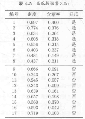
data_path = r"3.3\watermelon3_0_Ch.csv"
#
data = pd.read_csv(data_path).values
is_good = data[:, 9] == "是"
is_bad = data[:, 9] == "否"
X = data[:, 7:9].astype(float)
y = data[:, 9]
y[y == "是"] = 1
y[y == "否"] = 0
y = y.astype(int)
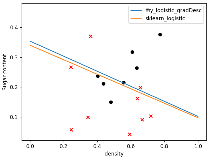
plt.scatter(data[:, 7][is_good], data[:, 8][is_good], c="k", marker="o")
plt.scatter(data[:, 7][is_bad], data[:, 8][is_bad], c="r", marker="x")
plt.xlabel("密度")
plt.ylabel("含糖量")
# 可视化模型结果
beta = logistic_model(
X, y, print_cost=True, method="gradDesc", learning_rate=0.3, num_iterations=1000
)
w1, w2, intercept = beta
x1 = np.linspace(0, 1)
y1 = -(w1 * x1 + intercept) / w2
(ax1,) = plt.plot(x1, y1, label=r"my_logistic_gradDesc")
lr = linear_model.LogisticRegression(
solver="lbfgs", C=1000
) # 注意sklearn的逻辑回归中,C越大表示正则化程度越低。
lr.fit(X, y)
lr_beta = np.c_[lr.coef_, lr.intercept_]
print(J_cost(X, y, lr_beta))
# 可视化sklearn LogisticRegression 模型结果
w1_sk, w2_sk = lr.coef_[0, :]
x2 = np.linspace(0, 1)
y2 = -(w1_sk * x2 + lr.intercept_) / w2
(ax2,) = plt.plot(x2, y2, label=r"sklearn_logistic")
plt.legend(loc="upper right")
plt.show()
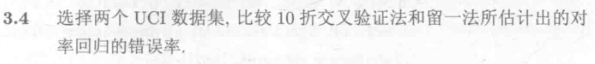
3.4:
解:
import numpy as np
from sklearn import linear_model
from sklearn.model_selection import LeaveOneOut
from sklearn.model_selection import cross_val_score

data_path = r"3.4\\Transfusion.txt"

data = np.loadtxt(data_path, delimiter=",").astype(int)

X = data[:, :4]
y = data[:, 4]

m, n = X.shape

# normalization
X = (X - X.mean(0)) / X.std(0)

# shuffle
index = np.arange(m)
np.random.shuffle(index)

X = X[index]
y = y[index]

# 使用sklarn 中自带的api先
# k-10 cross validation
lr = linear_model.LogisticRegression(C=2)

score = cross_val_score(lr, X, y, cv=10)

print("10折交叉验证_sklarn 中自带的api:", score.mean())

# LOO
loo = LeaveOneOut()

accuracy = 0
for train, test in loo.split(X, y):
    lr_ = linear_model.LogisticRegression(C=2)
    X_train = X[train]
    X_test = X[test]
    y_train = y[train]
    y_test = y[test]
    lr_.fit(X_train, y_train)

    accuracy += lr_.score(X_test, y_test)

print("留一法_sklarn 中自带的api:", accuracy / m)

# 两者结果几乎一样

# 自己写一个试试
# k-10
# 这里就没考虑最后几个样本了。
num_split = int(m / 10)
score_my = []
for i in range(10):
    lr_ = linear_model.LogisticRegression(C=2)
    test_index = range(i * num_split, (i + 1) * num_split)
    X_test_ = X[test_index]
    y_test_ = y[test_index]

    X_train_ = np.delete(X, test_index, axis=0)
    y_train_ = np.delete(y, test_index, axis=0)

    lr_.fit(X_train_, y_train_)

    score_my.append(lr_.score(X_test_, y_test_))

print("10折交叉验证_手搓:", np.mean(score_my))

# LOO
score_my_loo = []
for i in range(m):
    lr_ = linear_model.LogisticRegression(C=2)
    X_test_ = X[i, :]
    y_test_ = y[i]

    X_train_ = np.delete(X, i, axis=0)
    y_train_ = np.delete(y, i, axis=0)

    lr_.fit(X_train_, y_train_)

    score_my_loo.append(int(lr_.predict(X_test_.reshape(1, -1)) == y_test_))

print("留一法_手搓:", np.mean(score_my_loo))

# 结果都是类似
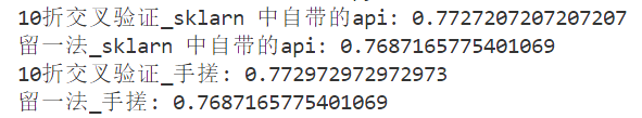
3.5:
![]()
解:
import numpy as np
import pandas as pd
from matplotlib import pyplot as plt


class LDA(object):

    def fit(self, X_, y_, plot_=False):
        pos = y_ == 1
        neg = y_ == 0
        X0 = X_[neg]
        X1 = X_[pos]

        u0 = X0.mean(0, keepdims=True)  # (1, n)
        u1 = X1.mean(0, keepdims=True)

        sw = np.dot((X0 - u0).T, X0 - u0) + np.dot((X1 - u1).T, X1 - u1)
        w = np.dot(np.linalg.inv(sw), (u0 - u1).T).reshape(1, -1)  # (1, n)

        if plot_:
            fig, ax = plt.subplots()
            ax.spines["right"].set_color("none")
            ax.spines["top"].set_color("none")
            ax.spines["left"].set_position(("data", 0))
            ax.spines["bottom"].set_position(("data", 0))

            plt.scatter(X1[:, 0], X1[:, 1], c="k", marker="o", label="good")
            plt.scatter(X0[:, 0], X0[:, 1], c="r", marker="x", label="bad")

            plt.xlabel("density", labelpad=1)
            plt.ylabel("Sugar content")
            plt.legend(loc="upper right")

            x_tmp = np.linspace(-0.05, 0.15)
            y_tmp = x_tmp * w[0, 1] / w[0, 0]
            plt.plot(x_tmp, y_tmp, "#808080", linewidth=1)

            wu = w / np.linalg.norm(w)

            # 正负样板店
            X0_project = np.dot(X0, np.dot(wu.T, wu))
            plt.scatter(X0_project[:, 0], X0_project[:, 1], c="r", s=15)
            for i in range(X0.shape[0]):
                plt.plot(
                    [X0[i, 0], X0_project[i, 0]],
                    [X0[i, 1], X0_project[i, 1]],
                    "--r",
                    linewidth=1,
                )

            X1_project = np.dot(X1, np.dot(wu.T, wu))
            plt.scatter(X1_project[:, 0], X1_project[:, 1], c="k", s=15)
            for i in range(X1.shape[0]):
                plt.plot(
                    [X1[i, 0], X1_project[i, 0]],
                    [X1[i, 1], X1_project[i, 1]],
                    "--k",
                    linewidth=1,
                )

            # 中心点的投影
            u0_project = np.dot(u0, np.dot(wu.T, wu))
            plt.scatter(u0_project[:, 0], u0_project[:, 1], c="#FF4500", s=60)
            u1_project = np.dot(u1, np.dot(wu.T, wu))
            plt.scatter(u1_project[:, 0], u1_project[:, 1], c="#696969", s=60)

            ax.annotate(
                r"u0 Projection point",
                xy=(u0_project[:, 0], u0_project[:, 1]),
                xytext=(u0_project[:, 0] - 0.2, u0_project[:, 1] - 0.1),
                size=13,
                va="center",
                ha="left",
                arrowprops=dict(
                    arrowstyle="->",
                    color="k",
                ),
            )

            ax.annotate(
                r"u1 Projection point",
                xy=(u1_project[:, 0], u1_project[:, 1]),
                xytext=(u1_project[:, 0] - 0.1, u1_project[:, 1] + 0.1),
                size=13,
                va="center",
                ha="left",
                arrowprops=dict(
                    arrowstyle="->",
                    color="k",
                ),
            )
            plt.axis("equal")  # 两坐标轴的单位刻度长度保存一致
            plt.show()

        self.w = w
        self.u0 = u0
        self.u1 = u1
        return self

    def predict(self, X):
        project = np.dot(X, self.w.T)

        wu0 = np.dot(self.w, self.u0.T)
        wu1 = np.dot(self.w, self.u1.T)

        return (np.abs(project - wu1) < np.abs(project - wu0)).astype(int)


if __name__ == "__main__":
    data_path = r"3.3\watermelon3_0_Ch.csv"

    data = pd.read_csv(data_path).values

    X = data[:, 7:9].astype(float)
    y = data[:, 9]

    y[y == "是"] = 1
    y[y == "否"] = 0
    y = y.astype(int)

    lda = LDA()
    lda.fit(X, y, plot_=True)
    print(lda.predict(X))  # 和逻辑回归的结果一致
    print(y)
3.6:

解:
引入核函数,原书p137,有关于核线性判别分析的介绍。
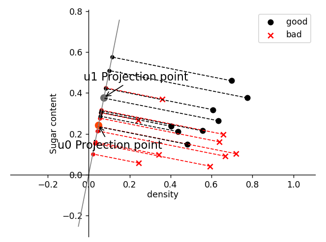
3.7:

解:
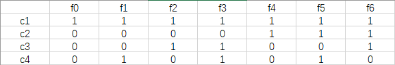
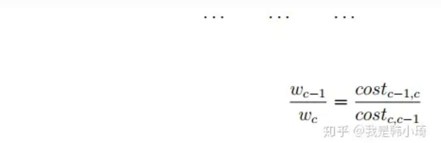
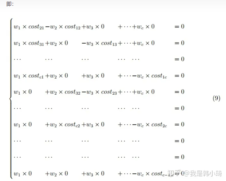
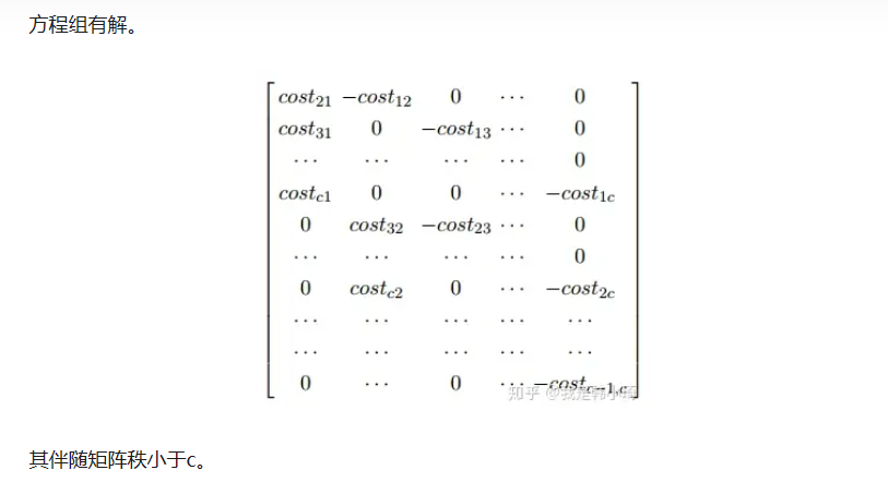
原论文中给出了构造编码的几种方法。其中一个是:
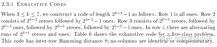
回到题目上,在类别为4时,其可行的编码有7种,按照上述方法有:

3.8:

解:
3.9:

解:
书中提到,对于OvR,MvM来说,由于对每个类进行了相同的处理,其拆解出的二分类任务中类别不平衡的影响会相互抵消,因此通常不需要专门处理。以ECOC编码为例,每个生成的二分类器会将所有样本分成较为均衡的二类,使类别不平衡的影响减小。当然拆解后仍然可能出现明显的类别不平衡现象,比如一个超级大类和一群小类。
3.10:

解:
参考文献:
机器学习(周志华)课后习题——第三章——线性模型 - 知乎 (zhihu.com)


 2194
2194

 被折叠的 条评论
为什么被折叠?
被折叠的 条评论
为什么被折叠?
 到【灌水乐园】发言


