


简述
由于科技论文老师要求阅读Gans论文并在网上找到类似的代码来学习。
代码来源
https://github.com/MorvanZhou/PyTorch-Tutorial/blob/master/tutorial-contents/406_GAN.py
代码含义概览
这个大致讲讲这个代码实现了什么。
这个模型的输入为:一些数据夹杂在
x
2
x^2
x2和
2
x
2
+
1
2x^2+1
2x2+1这个两个函数之间的一些数据。这个用线性函数的随机生成来生成这个东西
输出: 这是一个生成模型,生成模型的结果就是生成通过上面的输入数据输出这样的数据来画一条曲线
-
我们每次只取15个在x方向上等距的点。然后画出这条曲线来。
经过学习之后,我们要求这个模型能自己画出一条在其中的曲线来。 -
当然,由于我们设置的区间是有弧线的,即区间的概率上是有偏差的。经过足够多的拟合,有较高的概率使得整个模型画出来的曲线也是一个弧线。
代码分段解释
导入包:
import torch
import torch.nn as nn
import numpy as np
import matplotlib.pyplot as plt
设置参数:
- LR_G:生成器的学习率
- LR_D:判别器的学习率
- N_IDEAS:生成器的启发因子(就是生成器这个神经网络的初始输入层的节点数)
- ART_COMPONENTS:观测节点–每次用于画线的那些输出点的数量
- BATCH_SIZE:其实是输入数据的数量。
- PAINT_POINTS :就是把重复的那么多数据(将x区间等分为观测节点数量等分的x节点)叠起来而已。这样之后就直接代入就可以知道数据了。
BATCH_SIZE = 64
LR_G = 0.0001  # learning rate for generator
LR_D = 0.0001  # learning rate for discriminator
N_IDEAS = 5  # think of this as number of ideas for generating an art work (Generator)
ART_COMPONENTS = 15  # it could be total point G can draw in the canvas
PAINT_POINTS = np.vstack([np.linspace(-1, 1, ART_COMPONENTS) for _ in range(BATCH_SIZE)])
给出标准数据:
这个函数,会给出特定规模的标准数据
- 先创建一个(BATCH_SIZE,1)规模的来自于(1,2)均匀分布的随机数。
- 再用这个数据构建 a ∗ x 2 + ( a − 1 ) a*x ^2 + (a - 1) a∗x2+(a−1) 其中a来自于 ( 1 , 2 ) (1,2) (1,2)的均匀分布。然后有BATCH_SIZE 个结果,所以,我们会在前面说到,这个参数表示输入集合的大小
def artist_works():  # painting from the famous artist (real target)
    a = np.random.uniform(1, 2, size=BATCH_SIZE)[:, np.newaxis]
    paintings = a * np.power(PAINT_POINTS, 2) + (a - 1)
    paintings = torch.from_numpy(paintings).float()
    return paintings
构建模型:
搭建神经网络
- 这里搭建的神经网络,只需要构建映射层就好了。
- 生成器模型:先通过一个线性函数构建一个从N_IDEAS到128的映射。再通过激活函数ReLU()函数来做一个映射。最后,再用一个线性函数搭建从128到观测点的映射。(这些映射都是用矩阵乘法来实现的,所以,其实参数空间是三个不同的矩阵)
- 判别式模型:先通过一个观测点的到128的模型。再通过一个ReLU激活函数。之后,再用一个线性函数使得从128到1维度。一维就是常数,再做一个sigmoid的激活函数映射到 ( 0 , 1 ) (0,1) (0,1)空间。表示概率。
G = nn.Sequential(  # Generator
    nn.Linear(N_IDEAS, 128),  # random ideas (could from normal distribution)
    nn.ReLU(),
    nn.Linear(128, ART_COMPONENTS),  # making a painting from these random ideas
)

D = nn.Sequential(  # Discriminator
    nn.Linear(ART_COMPONENTS, 128),  # receive art work either from the famous artist or a newbie like G
    nn.ReLU(),
    nn.Linear(128, 1),
    nn.Sigmoid(),  # tell the probability that the art work is made by artist
)
构建优化器
opt_D = torch.optim.Adam(D.parameters(), lr=LR_D)
opt_G = torch.optim.Adam(G.parameters(), lr=LR_G)
构建了两个优化器。其实就是把对应模型的参数放进来了而已,之后,再设置一下学习率。
这里采用的是Adam模型来做优化。
迭代细节
其实这上面应该还有一些画图而加上的函数,但是对于模型不是很重要,这里就不看了。最后会有一个整体的模型。
for step in range(10000):
明显看出,使用了10000次的迭代。
- 先调用标准数据生成函数,生成标准数据。
- 再用pytorch的随机数来生特定大小的生成器启发因子。
- 之后,再把这个随机数丢给生成器。
- 明显,通过这样的训练,其实逐渐的训练这个生成器模型,在随机给输入的情况下,渐渐掌握输出正确的结果(个人感觉这里有提高的可能)
artist_paintings = artist_works()  # real painting from artist
G_ideas = torch.randn(BATCH_SIZE, N_IDEAS)  # random ideas
G_paintings = G(G_ideas)  # fake painting from G (random ideas)
再把假画和真画都丢给判别式模型。给出一个概率来。
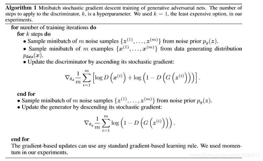
之后构建两个模型的交叉熵,需要降低的损失函数
D_loss = - torch.mean(torch.log(prob_artist0) + torch.log(1. - prob_artist1))
G_loss = torch.mean(torch.log(1. - prob_artist1))
这个其实是根据论文中的公式给出的。
- 注意到,这里跟下面算法中给出的梯度是相同的。就是前面少了个系数,但是有没系数,对于这个不影响的。
其实上面只是把整个模型搭建起来,其实都还没有运行的。
真正运行的部分是下面这里
opt_D.zero_grad()
D_loss.backward(retain_graph=True)  # reusing computational graph
opt_D.step()

opt_G.zero_grad()
G_loss.backward(retain_graph=True)
opt_G.step()
注意到,其实非常重复的。
- 第一步的zero_grad()函数:
原因:
In PyTorch, we need to set the gradients to zero before starting to do backpropragation because PyTorch accumulates the gradients on subsequent backward passes. This is convenient while training RNNs. So, the default action is to accumulate the gradients on every loss.backward() call.
在PyTorch中,我们需要设置这个梯度到0,在开始反向传播的训练之前,因为Pytorch会累积这个梯度在之后的反向传播过程中。这是非常方便的当训练RNNs的时候,所以默认就这么设置了。
Because of this, when you start your training loop, ideally you should zero out the gradients so that you do the parameter update correctly. Else the gradient would point in some other directions than the intended direction towards the minimum (or maximum, in case of maximization objectives).
由于这个,当你开始你的训练循环的时候,比较聪明的一点就是先把这个梯度设置为0,以确保你的训练的参数会是正确的。否则的话,这个梯度会指向一些其他地方(乱跑)
上面的解释来自于stackoverflow
https://stackoverflow.com/questions/48001598/why-is-zero-grad-needed-for-optimization
- 第二步:反向传播,这里设置保留整个图的情况下。
- 第三步:
.step()其实这个函数才真正表示这个模型被训练了。
画图
由于我们每次生成时候后,其实都是生成了一个BATCH_SIZE个。但是我们一次画太多的图的话,会显得很丑,所以就只画第一个图就好了。
这里取模的原因就在于避免画太多的图,导致耗费太多资源。
    if step % 500 == 0:  # plotting
        plt.cla()
        plt.plot(PAINT_POINTS[0], G_paintings.data.numpy()[0], c='#4AD631', lw=3, label='Generated painting', )
        # 2x^2 + 1
        plt.plot(PAINT_POINTS[0], 2 * np.power(PAINT_POINTS[0], 2) + 1, c='#74BCFF', lw=3, label='upper bound')
        # x^2
        plt.plot(PAINT_POINTS[0], 1 * np.power(PAINT_POINTS[0], 2) + 0, c='#FF9359', lw=3, label='lower bound')
        plt.text(-.5, 2.3, 'D accuracy=%.2f (0.5 for D to converge)' % prob_artist0.data.numpy().mean(),
                 fontdict={'size': 13})
        plt.text(-.5, 2, 'D score= %.2f (-1.38 for G to converge)' % -D_loss.data.numpy(), fontdict={'size': 13})
        plt.ylim((0, 3))
        plt.legend(loc='upper right', fontsize=10)
        plt.draw()
        plt.pause(0.01)
全部代码:
import torch
import torch.nn as nn
import numpy as np
import matplotlib.pyplot as plt

# Hyper Parameters
BATCH_SIZE = 64
LR_G = 0.0001  # learning rate for generator
LR_D = 0.0001  # learning rate for discriminator
N_IDEAS = 5  # think of this as number of ideas for generating an art work (Generator)
ART_COMPONENTS = 15  # it could be total point G can draw in the canvas
PAINT_POINTS = np.vstack([np.linspace(-1, 1, ART_COMPONENTS) for _ in range(BATCH_SIZE)])


def artist_works():  # painting from the famous artist (real target)
    a = np.random.uniform(1, 2, size=BATCH_SIZE)[:, np.newaxis]
    paintings = a * np.power(PAINT_POINTS, 2) + (a - 1)
    paintings = torch.from_numpy(paintings).float()
    return paintings


G = nn.Sequential(  # Generator
    nn.Linear(N_IDEAS, 128),  # random ideas (could from normal distribution)
    nn.ReLU(),
    nn.Linear(128, ART_COMPONENTS),  # making a painting from these random ideas
)

D = nn.Sequential(  # Discriminator
    nn.Linear(ART_COMPONENTS, 128),  # receive art work either from the famous artist or a newbie like G
    nn.ReLU(),
    nn.Linear(128, 1),
    nn.Sigmoid(),  # tell the probability that the art work is made by artist
)

opt_D = torch.optim.Adam(D.parameters(), lr=LR_D)
opt_G = torch.optim.Adam(G.parameters(), lr=LR_G)

plt.ion()  # something about continuous plotting

for step in range(10000):
    artist_paintings = artist_works()  # real painting from artist
    G_ideas = torch.randn(BATCH_SIZE, N_IDEAS)  # random ideas
    G_paintings = G(G_ideas)  # fake painting from G (random ideas)

    prob_artist0 = D(artist_paintings)  # D try to increase this prob
    prob_artist1 = D(G_paintings)  # D try to reduce this prob

    D_loss = - torch.mean(torch.log(prob_artist0) + torch.log(1. - prob_artist1))
    G_loss = torch.mean(torch.log(1. - prob_artist1))

    opt_D.zero_grad()
    D_loss.backward(retain_graph=True)  # reusing computational graph
    opt_D.step()

    opt_G.zero_grad()
    G_loss.backward(retain_graph=True)
    opt_G.step()

    if step % 500 == 0:  # plotting
        plt.cla()
        plt.plot(PAINT_POINTS[0], G_paintings.data.numpy()[0], c='#4AD631', lw=3, label='Generated painting', )
        # 2x^2 + 1
        plt.plot(PAINT_POINTS[0], 2 * np.power(PAINT_POINTS[0], 2) + 1, c='#74BCFF', lw=3, label='upper bound')
        # x^2
        plt.plot(PAINT_POINTS[0], 1 * np.power(PAINT_POINTS[0], 2) + 0, c='#FF9359', lw=3, label='lower bound')
        plt.text(-.5, 2.3, 'D accuracy=%.2f (0.5 for D to converge)' % prob_artist0.data.numpy().mean(),
                 fontdict={'size': 13})
        plt.text(-.5, 2, 'D score= %.2f (-1.38 for G to converge)' % -D_loss.data.numpy(), fontdict={'size': 13})
        plt.ylim((0, 3))
        plt.legend(loc='upper right', fontsize=10)
        plt.draw()
        plt.pause(0.01)

plt.ioff()
plt.show()


 3816
3816


 被折叠的 条评论
为什么被折叠?
被折叠的 条评论
为什么被折叠?
 到【灌水乐园】发言


