第P8周：YOLOv5-C3模块实现

最新推荐文章于 2024-06-17 18:28:04 发布

骑猪玩狗

最新推荐文章于 2024-06-17 18:28:04 发布

阅读量489

点赞数 14

文章标签： YOLO

本文链接：https://blog.csdn.net/a536723241/article/details/135348595

版权

>- **🍨 本文为[🔗365天深度学习训练营](https://mp.weixin.qq.com/s/rbOOmire8OocQ90QM78DRA) 中的学习记录博客**
>- **🍖 原作者：[K同学啊 | 接辅导、项目定制](https://mtyjkh.blog.csdn.net/)**

一、前期准备

1. 设置GPU

import torch
import torch.nn as nn
import torchvision
from torchvision import transforms, datasets
import os,PIL,pathlib,warnings

warnings.filterwarnings("ignore")             #忽略警告信息

device = torch.device("cuda" if torch.cuda.is_available() else "cpu")
device

2. 导入数据

import os,PIL,random,pathlib

data_dir = 'F:/365data/P3/'
data_dir = pathlib.Path(data_dir)

data_paths  = list(data_dir.glob('*'))
classeNames = [str(path).split("\\")[3] for path in data_paths]
classeNames

transforms = transforms.Compose([
    transforms.Resize([224,224]),
    transforms.ToTensor(),
    transforms.Normalize(
        mean=[0.485,0.456,0.406],
        std=[0.229,0.224,0.225]
    )
])

total_dataset = datasets.ImageFolder('F:/365data/P3/',transform=transforms)
total_dataset

3. 划分数据集

train_size = int(0.8*len(total_dataset))
test_size = len(total_dataset) - train_size
train_dataset,test_dataset = torch.utils.data.random_split(total_dataset,[train_size,test_size])
train_dataset,test_dataset

batch_size = 4

train_dl = torch.utils.data.DataLoader(train_dataset,
                                       batch_size = batch_size,
                                       shuffle = True,
                                       num_workers = 1)
test_dl = torch.utils.data.DataLoader(test_dataset,
                                        batch_size = batch_size,
                                        shuffle = True,
                                        num_workers = 1)

for X, y in test_dl:
    print("Shape of X [N, C, H, W]: ", X.shape)
    print("Shape of y: ", y.shape, y.dtype)
    break

二、搭建包含C3模块的模型

1. 搭建模型

import torch.nn.functional as F

def autopad(k, p=None):  # kernel, padding
    # Pad to 'same'
    if p is None:
        p = k // 2 if isinstance(k, int) else [x // 2 for x in k]  # auto-pad
    return p

class Conv(nn.Module):
    # Standard convolution
    def __init__(self, c1, c2, k=1, s=1, p=None, g=1, act=True):  # ch_in, ch_out, kernel, stride, padding, groups
        super().__init__()
        self.conv = nn.Conv2d(c1, c2, k, s, autopad(k, p), groups=g, bias=False)
        self.bn = nn.BatchNorm2d(c2)
        self.act = nn.SiLU() if act is True else (act if isinstance(act, nn.Module) else nn.Identity())

    def forward(self, x):
        return self.act(self.bn(self.conv(x)))

class Bottleneck(nn.Module):
    # Standard bottleneck
    def __init__(self, c1, c2, shortcut=True, g=1, e=0.5):  # ch_in, ch_out, shortcut, groups, expansion
        super().__init__()
        c_ = int(c2 * e)  # hidden channels
        self.cv1 = Conv(c1, c_, 1, 1)
        self.cv2 = Conv(c_, c2, 3, 1, g=g)
        self.add = shortcut and c1 == c2

    def forward(self, x):
        return x + self.cv2(self.cv1(x)) if self.add else self.cv2(self.cv1(x))

class C3(nn.Module):
    # CSP Bottleneck with 3 convolutions
    def __init__(self, c1, c2, n=1, shortcut=True, g=1, e=0.5):  # ch_in, ch_out, number, shortcut, groups, expansion
        super().__init__()
        c_ = int(c2 * e)  # hidden channels
        self.cv1 = Conv(c1, c_, 1, 1)
        self.cv2 = Conv(c1, c_, 1, 1)
        self.cv3 = Conv(2 * c_, c2, 1)  # act=FReLU(c2)
        self.m = nn.Sequential(*(Bottleneck(c_, c_, shortcut, g, e=1.0) for _ in range(n)))

    def forward(self, x): # x是传播到最内层的函数
        return self.cv3(torch.cat((self.m(self.cv1(x)), self.cv2(x)), dim=1))

class model_K(nn.Module):
    def __init__(self):
        super(model_K, self).__init__()
        
        # 卷积模块
        self.Conv = Conv(3, 32, 3, 2) 
        
        # C3模块1
        self.C3_1 = C3(32, 64, 3, 2)
        
        # 全连接网络层，用于分类
        self.classifier = nn.Sequential(
            nn.Linear(in_features=802816, out_features=100),# 全连接层也可以压缩特征数
            nn.ReLU(),
            nn.Linear(in_features=100, out_features=4)
        )
        
    def forward(self, x):
        x = self.Conv(x)
        x = self.C3_1(x)
        x = torch.flatten(x, start_dim=1)
        x = self.classifier(x)

        return x

device = "cuda" if torch.cuda.is_available() else "cpu"
print("Using {} device".format(device))
    
model = model_K().to(device)
model

2. 查看模型详情

# 统计模型参数量以及其他指标
import torchsummary as summary
summary.summary(model, (3, 224, 224))

三、训练模型

1. 编写训练函数

# 训练循环
def train(dataloader, model, loss_fn, optimizer):
    size = len(dataloader.dataset)  # 训练集的大小
    num_batches = len(dataloader)   # 批次数目, (size/batch_size，向上取整)

    train_loss, train_acc = 0, 0  # 初始化训练损失和正确率
    
    for X, y in dataloader:  # 获取图片及其标签
        X, y = X.to(device), y.to(device)
        
        # 计算预测误差
        pred = model(X)          # 网络输出
        loss = loss_fn(pred, y)  # 计算网络输出和真实值之间的差距，targets为真实值，计算二者差值即为损失
        
        # 反向传播
        optimizer.zero_grad()  # grad属性归零
        loss.backward()        # 反向传播
        optimizer.step()       # 每一步自动更新
        
        # 记录acc与loss
        train_acc  += (pred.argmax(1) == y).type(torch.float).sum().item()
        train_loss += loss.item()
            
    train_acc  /= size
    train_loss /= num_batches

    return train_acc, train_loss

2. 编写测试函数

def test (dataloader, model, loss_fn):
    size        = len(dataloader.dataset)  # 测试集的大小
    num_batches = len(dataloader)          # 批次数目, (size/batch_size，向上取整)
    test_loss, test_acc = 0, 0
    
    # 当不进行训练时，停止梯度更新，节省计算内存消耗
    with torch.no_grad():
        for imgs, target in dataloader:
            imgs, target = imgs.to(device), target.to(device)
            
            # 计算loss
            target_pred = model(imgs)
            loss        = loss_fn(target_pred, target)
            
            test_loss += loss.item()
            test_acc  += (target_pred.argmax(1) == target).type(torch.float).sum().item()

    test_acc  /= size
    test_loss /= num_batches

    return test_acc, test_loss

3. 正式训练

import copy

optimizer  = torch.optim.Adam(model.parameters(), lr= 1e-4)
loss_fn    = nn.CrossEntropyLoss() # 创建损失函数

epochs     = 20

train_loss = []
train_acc  = []
test_loss  = []
test_acc   = []

best_acc = 0    # 设置一个最佳准确率，作为最佳模型的判别指标

for epoch in range(epochs):
    
    model.train()
    epoch_train_acc, epoch_train_loss = train(train_dl, model, loss_fn, optimizer)
    
    model.eval()
    epoch_test_acc, epoch_test_loss = test(test_dl, model, loss_fn)
    
    # 保存最佳模型到 best_model
    if epoch_test_acc > best_acc:
        best_acc   = epoch_test_acc
        best_model = copy.deepcopy(model)
    
    train_acc.append(epoch_train_acc)
    train_loss.append(epoch_train_loss)
    test_acc.append(epoch_test_acc)
    test_loss.append(epoch_test_loss)
    
    # 获取当前的学习率
    lr = optimizer.state_dict()['param_groups'][0]['lr']
    
    template = ('Epoch:{:2d}, Train_acc:{:.1f}%, Train_loss:{:.3f}, Test_acc:{:.1f}%, Test_loss:{:.3f}, Lr:{:.2E}')
    print(template.format(epoch+1, epoch_train_acc*100, epoch_train_loss, 
                          epoch_test_acc*100, epoch_test_loss, lr))
    
# 保存最佳模型到文件中
PATH = 'F:/365data/P8best_model.pth'  # 保存的参数文件名
torch.save(model.state_dict(), PATH)

print('Done')

Epoch: 1, Train_acc:67.8%, Train_loss:1.356, Test_acc:83.6%, Test_loss:0.483, Lr:1.00E-04
Epoch: 2, Train_acc:89.1%, Train_loss:0.319, Test_acc:89.3%, Test_loss:0.370, Lr:1.00E-04
Epoch: 3, Train_acc:93.2%, Train_loss:0.188, Test_acc:91.6%, Test_loss:0.243, Lr:1.00E-04
Epoch: 4, Train_acc:96.2%, Train_loss:0.137, Test_acc:88.4%, Test_loss:0.351, Lr:1.00E-04
Epoch: 5, Train_acc:96.2%, Train_loss:0.143, Test_acc:88.0%, Test_loss:0.506, Lr:1.00E-04
Epoch: 6, Train_acc:97.1%, Train_loss:0.108, Test_acc:78.2%, Test_loss:1.285, Lr:1.00E-04
Epoch: 7, Train_acc:95.7%, Train_loss:0.164, Test_acc:86.7%, Test_loss:0.515, Lr:1.00E-04
Epoch: 8, Train_acc:99.1%, Train_loss:0.043, Test_acc:89.3%, Test_loss:0.414, Lr:1.00E-04
Epoch: 9, Train_acc:99.6%, Train_loss:0.017, Test_acc:89.3%, Test_loss:0.337, Lr:1.00E-04
Epoch:10, Train_acc:99.0%, Train_loss:0.031, Test_acc:88.9%, Test_loss:0.451, Lr:1.00E-04
Epoch:11, Train_acc:99.8%, Train_loss:0.009, Test_acc:90.2%, Test_loss:0.312, Lr:1.00E-04
Epoch:12, Train_acc:100.0%, Train_loss:0.003, Test_acc:90.2%, Test_loss:0.393, Lr:1.00E-04
Epoch:13, Train_acc:99.8%, Train_loss:0.005, Test_acc:90.2%, Test_loss:0.525, Lr:1.00E-04
Epoch:14, Train_acc:96.9%, Train_loss:0.114, Test_acc:84.9%, Test_loss:0.716, Lr:1.00E-04
Epoch:15, Train_acc:97.0%, Train_loss:0.093, Test_acc:90.7%, Test_loss:0.868, Lr:1.00E-04
Epoch:16, Train_acc:98.1%, Train_loss:0.091, Test_acc:88.4%, Test_loss:0.523, Lr:1.00E-04
Epoch:17, Train_acc:99.0%, Train_loss:0.037, Test_acc:89.8%, Test_loss:0.531, Lr:1.00E-04
Epoch:18, Train_acc:98.7%, Train_loss:0.054, Test_acc:86.2%, Test_loss:1.328, Lr:1.00E-04
Epoch:19, Train_acc:98.3%, Train_loss:0.091, Test_acc:88.9%, Test_loss:0.851, Lr:1.00E-04
Epoch:20, Train_acc:99.1%, Train_loss:0.037, Test_acc:89.8%, Test_loss:0.710, Lr:1.00E-04
Done

将优化器换成SGD后的结果如下

Epoch: 1, Train_acc:74.2%, Train_loss:0.699, Test_acc:85.8%, Test_loss:0.451, Lr:1.00E-04
Epoch: 2, Train_acc:88.2%, Train_loss:0.378, Test_acc:87.6%, Test_loss:0.358, Lr:1.00E-04
Epoch: 3, Train_acc:93.3%, Train_loss:0.261, Test_acc:88.4%, Test_loss:0.335, Lr:1.00E-04
Epoch: 4, Train_acc:94.9%, Train_loss:0.195, Test_acc:88.4%, Test_loss:0.343, Lr:1.00E-04
Epoch: 5, Train_acc:97.4%, Train_loss:0.140, Test_acc:90.7%, Test_loss:0.325, Lr:1.00E-04
Epoch: 6, Train_acc:97.4%, Train_loss:0.118, Test_acc:89.8%, Test_loss:0.305, Lr:1.00E-04
Epoch: 7, Train_acc:97.7%, Train_loss:0.104, Test_acc:88.9%, Test_loss:0.280, Lr:1.00E-04
Epoch: 8, Train_acc:98.2%, Train_loss:0.106, Test_acc:88.9%, Test_loss:0.303, Lr:1.00E-04
Epoch: 9, Train_acc:98.7%, Train_loss:0.082, Test_acc:88.4%, Test_loss:0.295, Lr:1.00E-04
Epoch:10, Train_acc:98.8%, Train_loss:0.069, Test_acc:92.0%, Test_loss:0.280, Lr:1.00E-04
Epoch:11, Train_acc:99.2%, Train_loss:0.067, Test_acc:89.8%, Test_loss:0.275, Lr:1.00E-04
Epoch:12, Train_acc:99.6%, Train_loss:0.054, Test_acc:91.1%, Test_loss:0.279, Lr:1.00E-04
Epoch:13, Train_acc:99.2%, Train_loss:0.055, Test_acc:89.3%, Test_loss:0.275, Lr:1.00E-04
Epoch:14, Train_acc:99.4%, Train_loss:0.053, Test_acc:90.2%, Test_loss:0.260, Lr:1.00E-04
Epoch:15, Train_acc:99.8%, Train_loss:0.042, Test_acc:91.6%, Test_loss:0.273, Lr:1.00E-04
Epoch:16, Train_acc:99.7%, Train_loss:0.040, Test_acc:91.1%, Test_loss:0.274, Lr:1.00E-04
Epoch:17, Train_acc:99.4%, Train_loss:0.038, Test_acc:92.0%, Test_loss:0.285, Lr:1.00E-04
Epoch:18, Train_acc:99.9%, Train_loss:0.033, Test_acc:90.7%, Test_loss:0.277, Lr:1.00E-04
Epoch:19, Train_acc:99.8%, Train_loss:0.031, Test_acc:92.0%, Test_loss:0.261, Lr:1.00E-04
Epoch:20, Train_acc:99.7%, Train_loss:0.027, Test_acc:92.0%, Test_loss:0.289, Lr:1.00E-04
Done

与Adam方法相比，准确率有所提高，但是训练时间由1min增加到了5min，同时训练过程中波动幅度变小，准确率曲线更加平滑
在这里插入图片描述
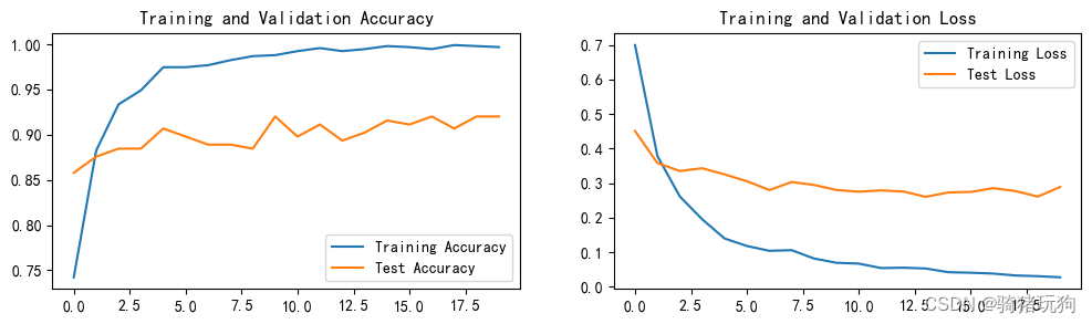
这也说明尽管Adam是一种集大成的方法，但有些时候使用SGD方法更好

四、结果可视化

1. Loss与Accuracy图

import matplotlib.pyplot as plt
#隐藏警告
import warnings
warnings.filterwarnings("ignore")               #忽略警告信息
plt.rcParams['font.sans-serif']    = ['SimHei'] # 用来正常显示中文标签
plt.rcParams['axes.unicode_minus'] = False      # 用来正常显示负号
plt.rcParams['figure.dpi']         = 100        #分辨率

epochs_range = range(epochs)

plt.figure(figsize=(12, 3))
plt.subplot(1, 2, 1)

plt.plot(epochs_range, train_acc, label='Training Accuracy')
plt.plot(epochs_range, test_acc, label='Test Accuracy')
plt.legend(loc='lower right')
plt.title('Training and Validation Accuracy')

plt.subplot(1, 2, 2)
plt.plot(epochs_range, train_loss, label='Training Loss')
plt.plot(epochs_range, test_loss, label='Test Loss')
plt.legend(loc='upper right')
plt.title('Training and Validation Loss')
plt.show()

在这里插入图片描述

2. 模型评估

best_model.eval()
epoch_test_acc, epoch_test_loss = test(test_dl, best_model, loss_fn)

epoch_test_acc, epoch_test_loss

# 查看是否与我们记录的最高准确率一致
epoch_test_acc