R语言实战：使用ggplot2绘制微生物组物种丰度堆叠柱状图

数据分析服务请访问以下链接：

文章发表技术服务，数据分析服务

数据和代码获取：请查看主页个人信息

在本篇文章中，我们将使用R语言来实现一个微生物组物种丰度堆叠柱状图。下面是一步步的过程，以及与之对应的代码：首先，我们需要导入在本示例中使用到的R包。这里我们使用了tidyverse，reshape2，phyloseq和ggsci。

Step 1: 导入所需的包

rm(list=ls())
pacman::p_load(tidyverse,reshape2,phyloseq,ggsci)

接下来，我们从phyloseq包中导入OTU表，并将OTU表与分类信息表合并为一个数据框。

Step 2: 读取数据

otufile <- system.file("extdata", "GP_otu_table_rand_short.txt.gz", package="phyloseq")
otu <- import_qiime(otufile)
head(otu@otu_table)[1:6, 1:10]

tax <- cbind(data.frame(otu@otu_table), data.frame(otu@tax_table)) %>% 
  rownames_to_column('OTU') %>% 
  select(OTU, Kingdom, Phylum, Class, Order, Family, Genus, Species)

# 将分类数据中的NA注释为“Unclassified”
tax[is.na(tax)] <- 'Unclassified'
head(tax)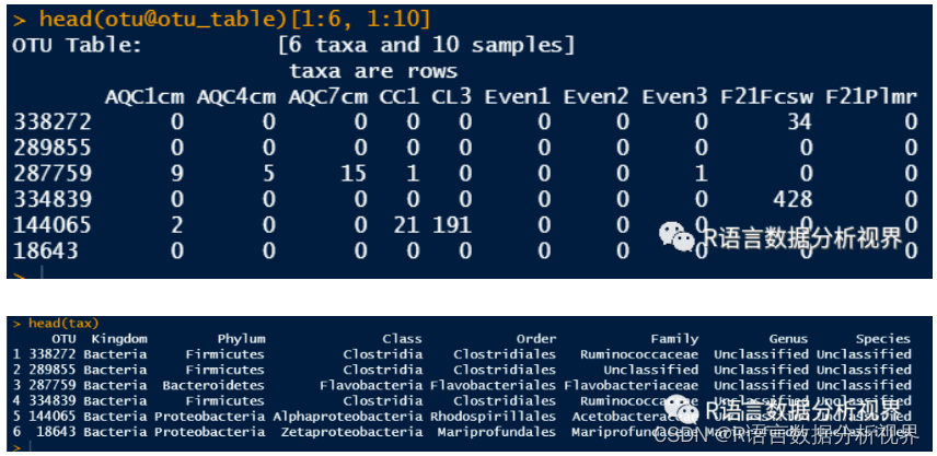

Step 3: 筛选表达量前9的OTU

top <- 
  data.frame(otu@otu_table) %>% 
  t() %>% 
  as.data.frame() %>% 
  summarise_if(is.numeric, sum, na.rm = TRUE) %>% 
  t() %>% 
  as.data.frame() %>% 
  set_names('SUM') %>% 
  arrange(desc(SUM)) %>% 
  rownames_to_column('OTU') %>% 
  head(9)
top

 在此步骤中，我们从整个OTU表中筛选出表达量前9的OTU，并保存它们的信息。

Step 4: 整理数据

otu_top <- 
  data.frame(otu@otu_table) %>% 
  rownames_to_column('OTU') %>% 
  filter(OTU %in% top$OTU) %>% 
  column_to_rownames('OTU') %>% 
  t() %>% 
  as.data.frame() %>% 
  rownames_to_column('sample')
otu_top

# 除了前9个表达量较高的OTU之外，其他被OTU定义为“Others”
otu_others <- 
  data.frame(otu@otu_table) %>% 
  rownames_to_column('OTU') %>% 
  filter(! OTU %in% rownames(top)) %>% 
  summarise_if(is.numeric, sum, na.rm = TRUE) %>% 
  t() %>% 
  as.data.frame() %>% 
  set_names('Others') %>% 
  rownames_to_column('sample')
  head(otu_others)
  
# 接下来这步比较关键，在分类变量数据中加入Others。
tax_top <- 
  tax %>% 
  filter(OTU %in% top$OTU) %>% 
  column_to_rownames('OTU') %>% 
  t() %>% 
  as.data.frame() %>% 
  mutate(Others = 'Others') %>% 
  t() %>% 
  as.data.frame() %>% 
  rownames_to_column('OTU')
tax_top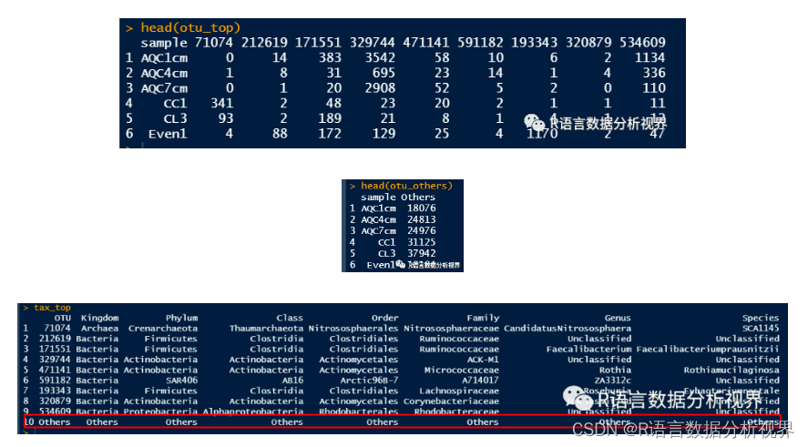

Step 5: 合并数据

# 绘图数据合并
dat <- 
  otu_top %>% 
  left_join(otu_others) %>% 
  melt(id.vars = 'sample') %>% 
  set_names(c('sample', 'OTU', 'value')) %>% 
  left_join(tax_top)
head(dat)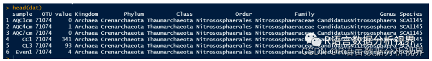

 

Step 6: 绘制OTU物种丰度堆叠柱状图

ggplot(dat, aes(sample, value, fill = OTU)) +
  geom_bar(stat="identity", position = 'fill')+
  xlab("") +
  ylab("") +
  theme_classic(base_size = 7) +
  scale_y_continuous(expand = c(0,0)) +
  ggtitle('OTU') +
  guides(fill=guide_legend(title=NULL)) +
  theme(axis.text.x=element_text(angle=45,vjust=1, hjust=1),
        legend.key.size = unit(10, "pt")) +
  ggsci::scale_fill_npg()

 

为了方便后续绘制不同分类级别的物种丰度堆叠柱状图，我们定义一个通用绘图函数pic()。

Step 7: 定义绘图函数

pic <- function(name){
  ggplot(dat, aes(sample, value, fill = dat[,name])) +
    geom_bar(stat="identity", position = 'fill')+
    xlab("") +
    ylab("") +
    theme_classic(base_size = 7) +
    scale_y_continuous(expand = c(0,0)) +
    ggtitle(name) +
    guides(fill=guide_legend(title=NULL)) +
    theme(axis.text.x=element_text(angle=45,vjust=1, hjust=1),
          legend.key.size = unit(10, "pt")) +
    ggsci::scale_fill_npg()
}

Step 8: 使用绘图函数绘制各分类级别的物种丰度堆叠柱状图

# pic('OTU')
pic('Kingdom')
pic('Phylum')
pic('Class')
pic('Order')
pic('Family')
pic('Genus')
pic('Species')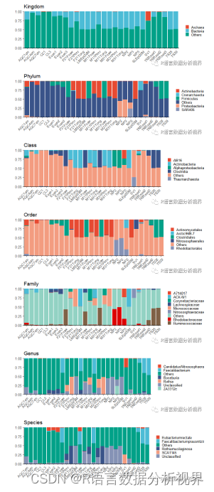

 好啦！本期分享到此结束，喜欢本期内容的童鞋们请点赞、关注、转发~