（7-3-03）TensorFlow自然语言处理实战：使用Seq2Seq模型实现机器翻译（3）

7.3.3  训练

开始训练数据，具体流程如下：

1. 将输入传送至编码器，编码器返回编码器输出和编码器隐藏层状态。
2. 将编码器输出、编码器隐藏层状态和解码器输入（即 开始标记）传送至解码器。
3. 解码器返回预测和解码器隐藏层状态。
4. 解码器隐藏层状态被传送回模型，预测被用于计算损失。
5. 使用 教师强制 （teacher forcing） 决定解码器的下一个输入。
6. 教师强制 是将 目标词 作为 下一个输入 传送至解码器的技术。
7. 最后一步是计算梯度，并将其应用于优化器和反向传播。

下面开始按照上述流程编写代码：

@tf.function
def train_step(inp, targ, enc_hidden):
  loss = 0

  with tf.GradientTape() as tape:
    enc_output, enc_hidden = encoder(inp, enc_hidden)

    dec_hidden = enc_hidden

    dec_input = tf.expand_dims([targ_lang.word_index['<start>']] * BATCH_SIZE, 1)

    # 教师强制 - 将目标词作为下一个输入
    for t in range(1, targ.shape[1]):
      # 将编码器输出 （enc_output） 传送至解码器
      predictions, dec_hidden, _ = decoder(dec_input, dec_hidden, enc_output)

      loss += loss_function(targ[:, t], predictions)

      # 使用教师强制
      dec_input = tf.expand_dims(targ[:, t], 1)

  batch_loss = (loss / int(targ.shape[1]))

  variables = encoder.trainable_variables + decoder.trainable_variables

  gradients = tape.gradient(loss, variables)

  optimizer.apply_gradients(zip(gradients, variables))

  return batch_loss

EPOCHS = 10

for epoch in range(EPOCHS):
  start = time.time()

  enc_hidden = encoder.initialize_hidden_state()
  total_loss = 0

  for (batch, (inp, targ)) in enumerate(dataset.take(steps_per_epoch)):
    batch_loss = train_step(inp, targ, enc_hidden)
    total_loss += batch_loss

    if batch % 100 == 0:
        print('Epoch {} Batch {} Loss {:.4f}'.format(epoch + 1,
                                                     batch,
                                                     batch_loss.numpy()))
  # 每 2 个周期（epoch），保存（检查点）一次模型
  if (epoch + 1) % 2 == 0:
    checkpoint.save(file_prefix = checkpoint_prefix)

  print('Epoch {} Loss {:.4f}'.format(epoch + 1,
                                      total_loss / steps_per_epoch))
  print('Time taken for 1 epoch {} sec\n'.format(time.time() - start))

执行后会输出：

Epoch 1 Batch 0 Loss 4.6508
Epoch 1 Batch 100 Loss 2.1923
Epoch 1 Batch 200 Loss 1.7957
Epoch 1 Batch 300 Loss 1.7889
Epoch 1 Loss 2.0564
Time taken for 1 epoch 28.358328819274902 sec

Epoch 2 Batch 0 Loss 1.5558
Epoch 2 Batch 100 Loss 1.5256
Epoch 2 Batch 200 Loss 1.4604
Epoch 2 Batch 300 Loss 1.3006
Epoch 2 Loss 1.4770
Time taken for 1 epoch 16.062172651290894 sec

Epoch 3 Batch 0 Loss 1.1928
Epoch 3 Batch 100 Loss 1.1909
Epoch 3 Batch 200 Loss 1.0559
Epoch 3 Batch 300 Loss 0.9279
Epoch 3 Loss 1.1305
Time taken for 1 epoch 15.620810270309448 sec

Epoch 4 Batch 0 Loss 0.8910
Epoch 4 Batch 100 Loss 0.7890
Epoch 4 Batch 200 Loss 0.8234
Epoch 4 Batch 300 Loss 0.8448
Epoch 4 Loss 0.8080
Time taken for 1 epoch 15.983836889266968 sec

Epoch 5 Batch 0 Loss 0.4728
Epoch 5 Batch 100 Loss 0.7090
Epoch 5 Batch 200 Loss 0.6280
Epoch 5 Batch 300 Loss 0.5421
Epoch 5 Loss 0.5710
Time taken for 1 epoch 15.588238716125488 sec

Epoch 6 Batch 0 Loss 0.4209
Epoch 6 Batch 100 Loss 0.3995
Epoch 6 Batch 200 Loss 0.4426
Epoch 6 Batch 300 Loss 0.4470
Epoch 6 Loss 0.4063
Time taken for 1 epoch 15.882423639297485 sec

Epoch 7 Batch 0 Loss 0.2503
Epoch 7 Batch 100 Loss 0.3373
Epoch 7 Batch 200 Loss 0.3342
Epoch 7 Batch 300 Loss 0.2955
Epoch 7 Loss 0.2938
Time taken for 1 epoch 15.601640939712524 sec

Epoch 8 Batch 0 Loss 0.1662
Epoch 8 Batch 100 Loss 0.1923
Epoch 8 Batch 200 Loss 0.2131
Epoch 8 Batch 300 Loss 0.2464
Epoch 8 Loss 0.2175
Time taken for 1 epoch 15.917790412902832 sec

Epoch 9 Batch 0 Loss 0.1450
Epoch 9 Batch 100 Loss 0.1351
Epoch 9 Batch 200 Loss 0.2102
Epoch 9 Batch 300 Loss 0.2188
Epoch 9 Loss 0.1659
Time taken for 1 epoch 15.727098941802979 sec

Epoch 10 Batch 0 Loss 0.0995
Epoch 10 Batch 100 Loss 0.1190
Epoch 10 Batch 200 Loss 0.1444
Epoch 10 Batch 300 Loss 0.1280
Epoch 10 Loss 0.1294
Time taken for 1 epoch 15.857161045074463 sec

7.3.4  翻译

评估函数evaluate(sentence)类似于训练循环，每个时间步的解码器输入是其先前的预测、隐藏层状态和编码器输出。当模型预测出现结束标记时停止预测，然后存储每个时间步的注意力权重。请注意，对于一个输入来说，编码器输出仅计算一次。评估函数evaluate(sentence)的代码如下：

def evaluate(sentence):
    attention_plot = np.zeros((max_length_targ, max_length_inp))

    sentence = preprocess_sentence(sentence)

    inputs = [inp_lang.word_index[i] for i in sentence.split(' ')]
    inputs = tf.keras.preprocessing.sequence.pad_sequences([inputs],
                                                           maxlen=max_length_inp,
                                                           padding='post')
    inputs = tf.convert_to_tensor(inputs)

    result = ''

    hidden = [tf.zeros((1, units))]
    enc_out, enc_hidden = encoder(inputs, hidden)

    dec_hidden = enc_hidden
    dec_input = tf.expand_dims([targ_lang.word_index['<start>']], 0)

    for t in range(max_length_targ):
        predictions, dec_hidden, attention_weights = decoder(dec_input,
                                                             dec_hidden,
                                                             enc_out)

        # 存储注意力权重以便后面制图
        attention_weights = tf.reshape(attention_weights, (-1, ))
        attention_plot[t] = attention_weights.numpy()

        predicted_id = tf.argmax(predictions[0]).numpy()

        result += targ_lang.index_word[predicted_id] + ' '

        if targ_lang.index_word[predicted_id] == '<end>':
            return result, sentence, attention_plot

        # 预测的 ID 被输送回模型
        dec_input = tf.expand_dims([predicted_id], 0)

    return result, sentence, attention_plot

# 注意力权重制图函数
def plot_attention(attention, sentence, predicted_sentence):
    fig = plt.figure(figsize=(10,10))
    ax = fig.add_subplot(1, 1, 1)
    ax.matshow(attention, cmap='viridis')

    fontdict = {'fontsize': 14}

    ax.set_xticklabels([''] + sentence, fontdict=fontdict, rotation=90)
    ax.set_yticklabels([''] + predicted_sentence, fontdict=fontdict)

    ax.xaxis.set_major_locator(ticker.MultipleLocator(1))
    ax.yaxis.set_major_locator(ticker.MultipleLocator(1))

    plt.show()

def translate(sentence):
    result, sentence, attention_plot = evaluate(sentence)

    print('Input: %s' % (sentence))
    print('Predicted translation: {}'.format(result))

    attention_plot = attention_plot[:len(result.split(' ')), :len(sentence.split(' '))]
    plot_attention(attention_plot, sentence.split(' '), result.split(' '))

接下来恢复最新的检查点，然后输入西班牙语“hace mucho frio aqu”进行验证，代码如下：

#恢复检查点目录 （checkpoint_dir） 中最新的检查点
checkpoint.restore(tf.train.latest_checkpoint(checkpoint_dir))
translate(u'hace mucho frio aqui.')

执行后会输出：

<tensorflow.python.training.tracking.util.CheckpointLoadStatus at 0x7f3d31e73f98>

Input: <start> hace mucho frio aqui . <end>
Predicted translation: it s very cold here . <end>

并调用注意力权重制图函数绘制翻译“hace mucho frio aqu”的翻译可视化图表，如图7-2所示。

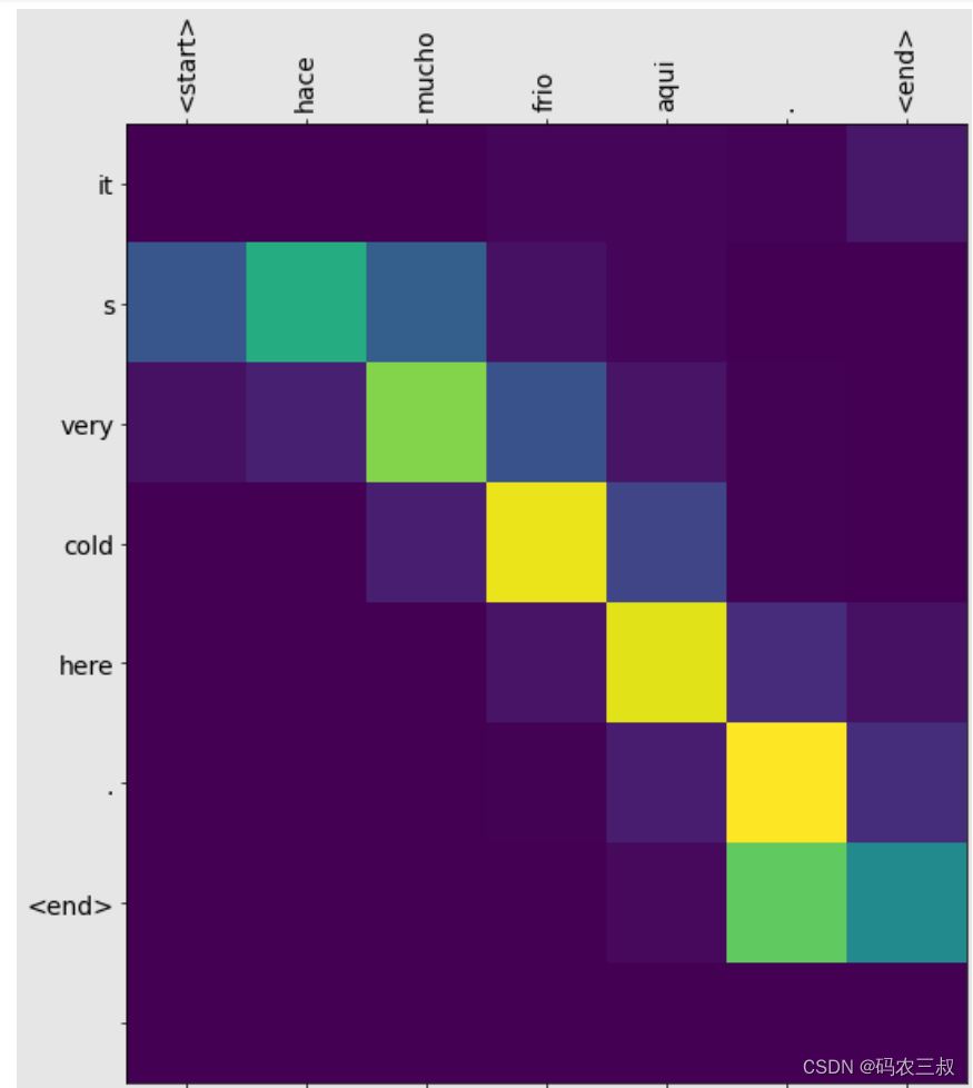
图7-2  “hace mucho frio aqu”的翻译可视化图表

输入西班牙语“esta es mi vida.”进行验证，代码如下：

translate(u'esta es mi vida.')

执行后会输出：

Input: <start> esta es mi vida . <end>

Predicted translation: this is my life . <end>

调用注意力权重制图函数绘制翻译“esta es mi vida.”的翻译可视化图表，如图7-3所示。

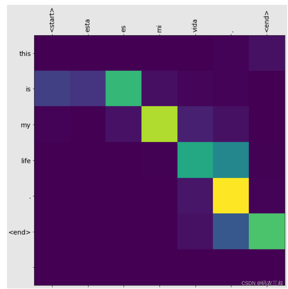
图7-3  “esta es mi vida.”的翻译可视化图表