Functional Data Analysis Notes - 3: Functional PCA

阅读材料：Ramsay, J.O., Silverman, B.W. (2005) Functional Data Analysis (2nd Edition) Section 8.1-8.6, 9.1-9.4.

1 Multivariate Principal Components Analysis

The basic idea of Principal Components Analysis is to transform a group of potentially correlated variables into a group of linearly uncorrelated variables through orthogonal transformation, and this group of variables after conversion are called principal components.

1.1 A little analysis

• Measure total variation in the data as total squared distance from center:
  $$\sum _{j=1}^d\sum _{i=1}^n(x_{ij}-{\bar{x}}_j{)}^2=trace[\Sigma ];$$
• If $x$ has covariance $\Sigma$, the variance of $u^{T}x$ is $u^T\Sigma u$;
• To maximize $u^T\Sigma u$ (or $u^{T}u$) we solve the eigen-equation
  $$\Sigma u=\lambda u;$$
• For $u^{T}u=1$, the closest multiple of $u$ to $x-\bar{x}$ is
  $$(u^{T}u{)}^{-1}(u^{T}x)u=(u^T(x-\bar{x}))u.$$

1.2 Mechanics of PCA

For an $n\times p$ data matrix with $n$ observations and $p$ attributions:

• Estimate the covariance matrix (using sample covariance matrix)
  $$\Sigma =\frac{1}{n-1}(X-\bar{X}{)}^T(X-\bar{X}),$$
  where $\bar{X}$ is the mean vector of the $p$ attributions of the data matrix $X$;
• Take the eigen-decomposition of $\Sigma$
  $$\Sigma =U^{T}DU=\sum d_{ii}{u}_i{u}_i^T;$$
  • Columns of $U$ are orthogonal; represent a new basis. Denoting the $i$^th column of $U$ by $u_i$;
  • $D$ is a diagonal matrix. Its entries ($d_{ii}$) (eigenvalues) give variances of data along corresponding directions $U$.
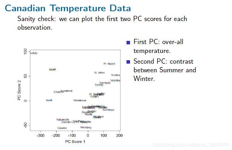
• Order $D$, $U$ in terms of decreasing $d_{ii}$;
• $(X-\bar{X}{)}^T{u}_i$ is the $i$^th principal component score.

2 Functional PCA

2.1 Re-interpretation

Instead of covariance matrix $\Sigma$, we have a surface $\sigma (s,t)$.

Re-interpret eigen-decomposition:

$$\Sigma =U^{T}DU=\sum d_{ii}{u}_i{u}_i^T.$$

For functions, this is the Karhunen-Loève decomposition:

$$\sigma (s,t)=\sum _{i=1}^{\infty }{d}_{ii}{\xi }_i(s){\xi }_i(t),$$

where

• $d_{ii}$ represents amount of variation in direction ${\xi }_i(t)$;
• $\int {\xi }_i(t{)}^{2}dt=I.$ (??)

For the collection of curves $x_i(t)$, $i=1,...,n$, we want to find the probe ${\xi }_1(t)$ that maximizes

$$Var[\int {\xi }_1(t)x_i(t)dt].$$

But we need to constrain $\int {\xi }_1(t{)}^{2}dt=1$.

For ${\xi }_2(t)$ we want to maximize the variance subject to the orthogonality condition
$$\int {\xi }_1(t){\xi }_2(t)dt=0$$

For ${\xi }_1,...,{\xi }_d$ best approximation to $x(t)$ is

$$\begin{array}{rl}\hat{x}(t)& =\bar{x}(t)+(\int (x(t)-\bar{x}(t)){\xi }_1(t)dt){\xi }_1(t)+...\\ & \\ & +(\int (x(t)-\bar{x}(t)){\xi }_d(t)dt){\xi }_d(t)\\ & \\ & =f_1{\xi }_1(t)+...+f_d{\xi }_d(t).\end{array}$$

which can be seen as a new basis!

For $\hat{y}=g_1{\xi }_1(t)+...+g_d{\xi }_d(t)$:

$$\int (\hat{x}(t)-\hat{y}(t){)}^{2}dt=\sum _{i=1}^d(f_i-g_i{)}^2.$$

The covariance surface can be decomposed:

$$\sigma (s,t)=\sum _{i=1}^{\infty }{d}_{ii}{\xi }_i(s){\xi }_i(t)$$

with the ${\xi }_i$ orthonormal.

• The ${\xi }_i(t)$ are the principal components; successively maximize $Va{r}_i[\int {\xi }_i(t)x_j(t)dt]$.
• $d_{ii}=Va{r}_i[\int {\xi }_i(t)x_j(t)dt]$.
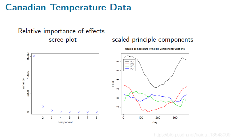
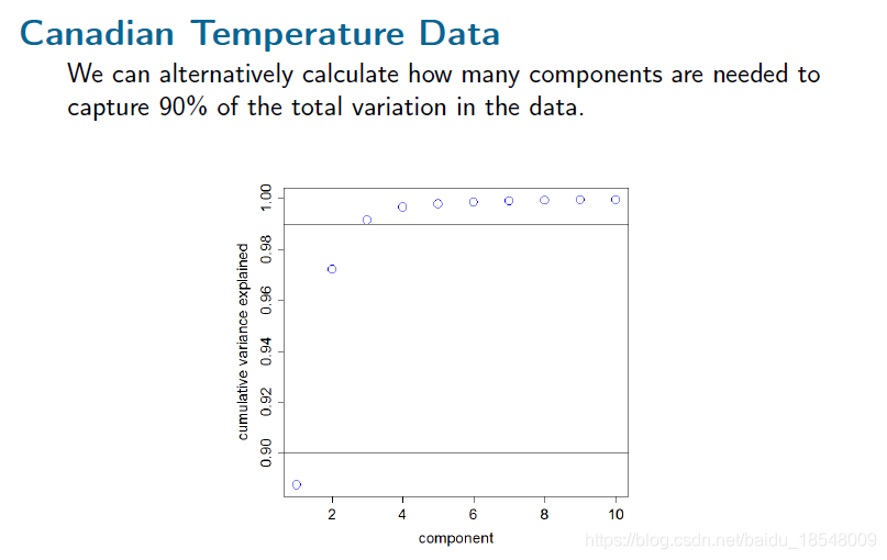
• $d_{ii}/\sum d_{ii}$ is proportion of variance explained.
• ${\xi }_1,...$ is a basis system specifically designed for the $x_i(t)$.
• Principal component scores are
  $$f_{ij}=\int {\xi }_i(t)[x_j(t)-\bar{x}(t)]dt$$
• Reconstrction of $x_i(t)$:
  $$x_i(t)=\bar{x}(t)+\sum _{j=1}^{\infty }{f}_{ij}{\xi }_j(t)$$

2.2 Computing FPCA

Components solve the eigen-equation:

$$\int \sigma (s,t){\xi }_i(t)dt=\lambda {\xi }_i(t)$$

Option 1:

1. take a fine grid $\mathbf{t}=[t_1,...,t_K]$
2. find the eigen-decomposition of $\Sigma (\mathbf{t},\mathbf{t})$
3. interpolate the eigenvectors

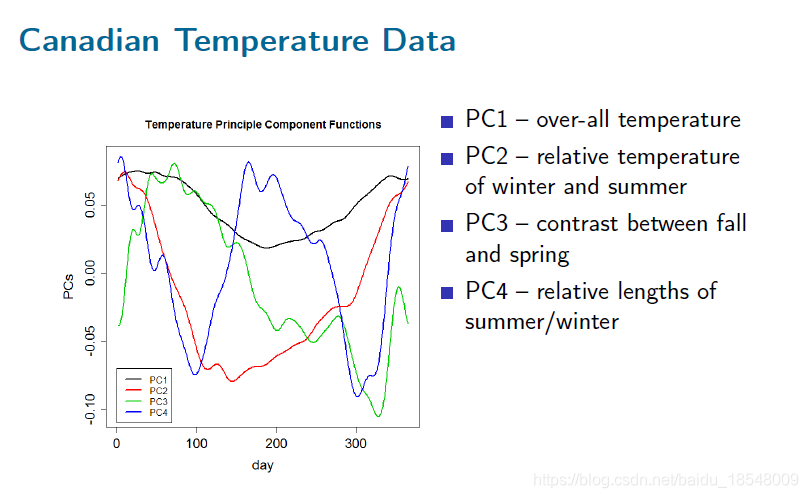
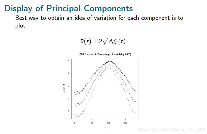
Option 2 (in fda library):

1. if the $x_i(t)$ have a common basis expansion, so must the eigen-functions;
2. can re-express eigen-equation in terms of co-efficients;
3. basis expansion will become apparent for smaller eigenvalues.

2.3 Varimax rotations

A set of principal components defines a subspace. Within that space, we can try to find a more interpretable basis. That amounts to a rotation of the coordinate axes.

The basic idea is to try to find coordinate system where PC loadings are either very large or very small.

The varimax criterion is

$$maximize\sum Var(u_i^2).$$

2.4 Summary

• PCA = means of summarizing high dimensional covariation;
• fPCA = extension to infinite-dimensional covariation;
• Representation terms of basis functions for fast(er) computation;
• Varimax rotations = focus on particular regions; nice display properties.

3 Smoothed PCA

3.1 A general perspective of PCA

For observations $x_1,x_2,...,x_n$ (vectors, functions, …), we want to find ${\xi }_1$ so that

$$\sum \Vert x_i-<x_i,{\xi }_1>{\xi }_1\Vert$$

is as small as possible.

$<x_i,{\xi }_1>$ is the best multiplier of ${\xi }_1$ to fit $x_i$.

Now we want ${\xi }_2$ to be the next best such that $<{\xi }_2,{\xi }_1>=0$.

3.1.1 Inner product

Vectors are otrhogonal if they intersect at right angles.

$\mathbf{x}$ and $\mathbf{y}$ are orthogonal if ${\mathbf{x}}^T\mathbf{y}=0$ (i.e. $\sum x_i{y}_i=0$).

In order to deal with $x(t)$ that are functions, multivariate functions, or mixed functions and scalars, we need a more general notation.

This will also help us understand smoothing a little more.

An inner produnct is a symmetric bilinear operator <., .> on a vector space $\mathcal{F}$ taking values in $\mathbb{R}$:

• $<x,y>=<y,x>$;
  (symmetry)
• $<ax,y>=a<x,y>$;
• $<x+y,z>=<x,z>+<y,z>$;
  (linearity for one element)
• $<x,x>>0$ with $x$ a non-zero vector.
  (positivity)

For example:

• Euclidean space: $<x,y>=x^{T}y$.
• ${\mathcal{L}}^2(\mathbb{R})$: $\int x(t)y(t)dt$.

Associated notion of distance or size:

$$\Vert x-y\Vert =<x-y,x-y>.$$

So to get to $x$ as close as possible in the direction $y$:

$$\underset{a}{\min }<x-ay,x-ay>,$$

which is solved at

$$a=<x,y>/<y,y>.$$

If $<y,y>=1$, $<x,y>$ is a measure of commonality.

If $<y,z>=0$ minimum of $\Vert x-ay-bz\Vert$ at

$$a=<x,y>,b=<x,z>.$$

3.1.2 Inner produncts and PCA

For a collection $x_1,x_2,...,x_n$, seek a probe $\xi$ to maximize

$$Var[<\xi ,x_i>].$$

Require $<{\xi }_i,{\xi }_j>={\delta }_{ij}$.

Implies optimal reconstruction:

$$\left[\begin{array}{ccc}<x_1,{\xi }_1>& \cdots & <x_1,{\xi }_d>\\ ⋮& & ⋮\\ <x_n,{\xi }_1>& \cdots & <x_n,{\xi }_d>\end{array}\right],$$

best summarization of $x_1,...,x_n$ with $d$ numbers.

3.1.3 Defining new inner products

For a multivariate function $\mathbf{x}(t)=(x_1(t),x_2(t))$.

A new inner product is

$$<(x_1,x_2),(y_1,y_2)>=<x_1,y_1>+<x_2,y_2>,$$

which can be check that this is a bilinear form.

Note that

$$<(x_1(t),x_2(t)),(y_1(t),y_2(t))>=0$$

does NOT imply

$$<x_1,y_1>=0and<x_2,y_2>=0$$

3.1.4 fPCA with multivariate functions

If we have $x_i(t)$ and $y_i(t)$, $i=1,...,n$.

Then we want to find $({\xi }_x(t),{\xi }_y(t))$ to maximize

$$Var[\int {\xi }_x(t)x_i(t)dt+\int {\xi }_y(t)y_i(t)dt].$$

This is like putting $x$ and $y$ together end-to-end:

$$z(t)=\{\begin{array}{l}x(t),t\le T\\ y(t),t>T\end{array}.$$

3.2 Smoothing and fPCA

When observed functions are rough, we may want the PCA to be smooth

• reduces high-frequency variation in the $x_i(t)$;
• provides better reconstruction of future $x_i(t)$.

We therefore want to find a way to impose smoothness on the principal components.

3.2.1 Including derivatives

Consider the multivariate function $(x(t),Lx(t))$, where $Lx(t)$ is the acceleration function (i.e. a function of $D^{n}x(t)$ ).

Inner product:

$$\begin{array}{rl}<x,y>& =<(x(t),Lx(t)),(y(t),Ly(t))>\\ & \\ & =\int x(t)y(t)dt+\lambda \int Lx(t)Ly(t)ndt.\end{array}$$

Smoothing:

• think of $\mathbf{y}=(y_1(t),y_2(t))=(y(t),0)$;
• try to fit with $\mathbf{x}=(x(t),Lx(t))$;
• but the norm is defined by the Sobolev inner product above.

3.2.2 A new measure of size

Usually, we measure size in the $L^2$ norm

$$\Vert \xi (t){\Vert }_2^2=\int \xi (t{)}^{2}dt.$$

But penalization methods implicitly use a *Sobolev norm:

$$\Vert \xi (t){\Vert }_L^2=\int \xi (t{)}^{2}dt+\lambda \int [L\xi (t){]}^{2}dt.$$

Search for the $\xi$ that maximizes

$$\frac{Var[\int \xi (t)x_i(t)dt]}{\Vert \xi (t){\Vert }_L^2}=\frac{Var[\int \xi (t)x_i(t)dt]}{\int \xi (t{)}^{2}dt+\lambda \int [L\xi (t){]}^{2}dt}.$$

3.2.3 Size and orthogonality

• As $\lambda$ increases, emphasize making $L\xi (t)$ small over maximizing the variance.
• Successive ${\xi }_i$ now satisfy
  $$\int {\xi }_i(t){\xi }_{j}dt+\lambda \int L{\xi }_i(t)L{\xi }_j(t)dt=0.$$
• Effectively “pretending” that $L{x}_i(t)=0$.
• Coeffiicients of best (in least-squares sense) fit no longer $\int {\xi }_i(t)x_j(t)dt$.
• Best fit coefficents now also depend on which eigenfunctions are used.

3.3 Summary

• Multivariate and Mixed PCs – like extending the vector;
• Need to think about weighting;
• Smoothing: may be done through a new inner product;
• Cross Validation: objective way to work out if smoothing is doing anything useful for you;
• Can use fPCA to help reconstruct partially-observed functions

4 Research papers

Liu, C., Ray, S., Hooker, G. and Friedl, M. (201), Functional principal component and factor analysis of spatially correlated data,
Statistics and Computing

Liu, C., Ray, S., Hooker, G. and Friedl, M. (2012), Functional factor analysis for periodic remote sensing data, The Annals of Applied Statistics 6(2), 601–624.

Paul, D. and Peng, J. (2011), Principal components analysis for sparsely observed correlated functional data using kernel smoothing method. Electronic Journal of Statistics (5).

Yao, F., Muller, H. and Wang, J. (2005), Functional data analysis for sparse longitudinal data, Journal of the American Statistical Association 100(470), 577–590.