pytorch入门示例

数据猴赛雷

已于 2022-03-16 10:46:49 修改

阅读量4.2k

点赞数

CC 4.0 BY-SA版权

分类专栏：神经网络文章标签： pytorch 深度学习机器学习

于 2022-03-11 11:37:17 首次发布

本文链接：https://blog.csdn.net/benben044/article/details/123415847

神经网络专栏收录该内容

62 篇文章

订阅专栏

本文详细介绍了如何使用PyTorch实现从Fashion MNIST数据集训练全连接网络和卷积神经网络，对比了两种模型在分类准确率上的表现，并展示了混淆矩阵和TensorBoard的使用。

第1步，导入相关的python包，并且下载训练集，其中训练集可以提前下载放到相应的目录下面。如果真的通过下面代码进行，将会相当耗时。

from torchvision import datasets, transforms
import torch
import torch.nn as nn
import torch.nn.functional as F
import torch.optim as optim


train_set = datasets.FashionMNIST('D:\\temp\\fashion_mnist',
                          train=True,
                          download=True,
                          transform=transforms.Compose([
                              transforms.ToTensor()
                          ])
)

当加载完图片数据，我们可以查看其中一张图片以验证加载是否正确。

import matplotlib.pyplot as plt
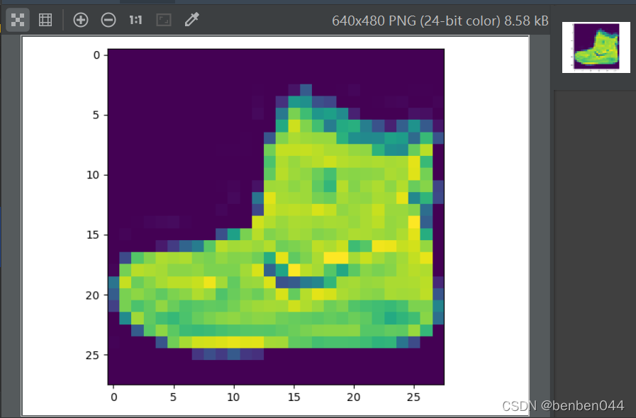
sample = next(iter(train_set))
plt.imshow(sample[0].squeeze())
plt.show()

sample的shape大小为[1,28,28]，而imshow显示则只能有[heigth, width]信息，所以通过squeeze()方法减小一个大小为1的轴。运行后显示如下：

第2步，以同样的方式，再加载测试集的数据。

test_set = datasets.FashionMNIST('D:\\temp\\fashion_mnist',
                          train=False,
                          download=True,
                          transform=transforms.Compose([
                              transforms.ToTensor()
                          ])
)

print('train_set size:', len(train_set), '   ,test_test size:', len(test_set))

打印训练集和测试集的数据，我们可以看到训练集有6万张图片，而测试集有1万张图片。

第3步，将训练集和测试集数据加载到loader中。loader可以提供批量加载、图片预处理，shuffle数据等功能。我们设定每一批的大小为100张，因为总共有6万张图片，所以总共有60000/100=60个批次。

train_loader = torch.utils.data.DataLoader(train_set, batch_size=100)
test_loader = torch.utils.data.DataLoader(test_set, batch_size=100)

batch = next(iter(train_loader))
images, labels = batch
print(images.shape)

查看每一批图片的shape为[100, 1, 28, 28]，分别对应[batch_size, channel_size, height, weight]的信息。

最简单的数据加载流程到此为止，下面我们将设计神经网络进行训练，并测试分类的效果。

第4步，设计全连接的网络结构

class FCNetwork(nn.Module):
    def __init__(self):
        super(FCNetwork, self).__init__()
        self.fc1 = nn.Linear(784, 200)
        self.fc2 = nn.Linear(200, 50)
        self.fc3 = nn.Linear(50, 10)

    def forward(self, x):
        x = F.relu(self.fc1(x))
        x = F.relu(self.fc2(x))
        x = self.fc3(x)
        return x

    def predict(self, x):
        logits = self.forward(x)
        return F.softmax(logits, dim=1)

以上是一个相对比较简单的全连接网络结构。

（1）nn.Linear要求输入的数据必须是二维的，需要将输入图像(28*28)展平后得到784列数据，输出为200列的数据，通过nn.Linear实现了两个不同维度（假如batch信息，比如之前是[100,784]的shape，后面是[100,200]的shape）的欧几里得空间数据的映射。

（2）因为fashion-mnist的分类结果是10个，所以最后一层需要输出10列的数据，每一列上的数据代表该分类的预测值。

（3）在预测环节，将测试值通过F.softmax()函数转化为概率值，此时10个分类的概率值之和为1.0

第5步，使用全连接网络训练模型，并且在测试集上验证模型的准确性。

fcNetwork = FCNetwork()
criterion = nn.CrossEntropyLoss()
optimizer = optim.Adam(fcNetwork.parameters(), lr=0.01)

epochs = 5
steps = 0
running_loss = 0
print_every = 60

for epoch in range(epochs):
    for images, labels in iter(train_loader):
        steps += 1
        input = images.view(-1, 784)

        optimizer.zero_grad()
        output = fcNetwork(input)
        loss = criterion(output, labels)
        loss.backward()
        optimizer.step()

        running_loss += loss.item()

    if steps % print_every == 0:
        accuracy = 0
        for ii, (images, labels) in enumerate(test_loader):
            inputs = images.view(-1, 784)
            preds = fcNetwork(inputs)
            accuracy += preds.argmax(dim=1).eq(labels).type_as(torch.FloatTensor()).mean()
        print("Epoch: {}/{}".format(epoch + 1, epochs),
              "Loss: {:.4f}".format(running_loss / print_every),
              "Test accuracy: {:.4f}".format(accuracy / (ii + 1)))
        running_loss = 0

（1）images的shape为[100, 1, 28, 28]，而nn.Linear()需要输入的格式为[batch_size, 784]，所以通过images.view(-1, 784)进行了转化，得到[100, 784]维度的数据。

（2）optimizer中的梯度信息是不断累加（链式求导）的，需要在每批数据训练前清空一下上次得到的梯度信息，避免不同批次间的grad相互干扰。

（3）loss.backward()是计算grad信息。

（4）optimizer.step()是根据第(3)的grad信息计算weight信息。

（5）preds.argmax(dim=1)可以获得预测值属于哪一类的信息。

（6）执行结果如下：

Epoch: 1/5 Loss: 5.1928 Test accuracy: 0.8200
Epoch: 2/5 Loss: 4.0105 Test accuracy: 0.8487
Epoch: 3/5 Loss: 3.7100 Test accuracy: 0.8498
Epoch: 4/5 Loss: 3.5857 Test accuracy: 0.8528
Epoch: 5/5 Loss: 3.4329 Test accuracy: 0.8570

第6步，使用CNN网络构建神经网络

class CNNNetwork(nn.Module):
    def __init__(self):
        super(CNNNetwork, self).__init__()
        self.conv1 = nn.Conv2d(1, 6, 5)
        self.conv2 = nn.Conv2d(6, 16, 5)
        self.fc1 = nn.Linear(16*4*4, 120)
        self.fc2 = nn.Linear(120, 84)
        self.fc3 = nn.Linear(84, 10)

    def forward(self, x):
        x = F.max_pool2d(F.relu(self.conv1(x)), (2,2))
        x = F.max_pool2d(F.relu(self.conv2(x)), 2)
        x = torch.flatten(x, start_dim=1)
        x = F.relu(self.fc1(x))
        x = F.relu(self.fc2(x))
        x = self.fc3(x)
        return x

    def predict(self, x):
        logits = self.forward(x)
        return F.softmax(logits, dim=1)

（1）nn.Conv2d(1， 6， 5)，卷积的输入需要是[batch, channel, heigth, width]格式的。其中1指的是输入图像是1通道的。6指的是有6个卷积核，每个卷积核都是(5,5)维度的。

（2）只有卷积网络需要有F.max_pool2d()池化操作，而全连接是不需要用池化操作的。

第7步，使用cnn网络训练模型

cnnNetwork = CNNNetwork()
criterion = nn.CrossEntropyLoss()
optimizer = optim.Adam(cnnNetwork.parameters(), lr=0.01)

epochs = 5
steps = 0
running_loss = 0
print_every = 60

for epoch in range(epochs):
    for images, labels in iter(train_loader):
        steps += 1

        optimizer.zero_grad()
        output = cnnNetwork(images)
        loss = criterion(output, labels)
        loss.backward()
        optimizer.step()

        running_loss += loss.item()

    if steps % print_every == 0:
        accuracy = 0
        for ii, (images, labels) in enumerate(test_loader):
            preds = cnnNetwork(images)
            accuracy += preds.argmax(dim=1).eq(labels).type_as(torch.FloatTensor()).mean()
        print("Epoch: {}/{}".format(epoch + 1, epochs),
              "Loss: {:.4f}".format(running_loss / print_every),
              "Test accuracy: {:.4f}".format(accuracy / (ii + 1)))
        running_loss = 0

运行后输出如下，可以看到使用cnn网络的准确率稍微高一点点。

Epoch: 1/5 Loss: 5.0865 Test accuracy: 0.8457
Epoch: 2/5 Loss: 3.6299 Test accuracy: 0.8417
Epoch: 3/5 Loss: 3.3446 Test accuracy: 0.8495
Epoch: 4/5 Loss: 3.2233 Test accuracy: 0.8719
Epoch: 5/5 Loss: 3.1051 Test accuracy: 0.8697

第8步，使用混淆矩阵查看预测结果

(images, labels) = next(iter(test_loader))
preds = cnnNetwork(images).argmax(dim=1)

from sklearn.metrics import confusion_matrix
cm = confusion_matrix(labels, preds)
print(cm)

取一批测试集数据校验结果，结果如下，可以看到每行的最大值基本上是沿着对角线走的，说明预测值基本上等于实际值。

[[ 8  0  0  0  0  0  0  0  0  0]
 [ 0 13  0  0  0  0  0  0  0  0]
 [ 0  0 13  1  0  0  0  0  0  0]
 [ 0  1  0  6  1  0  1  0  0  0]
 [ 0  0  2  0  6  0  2  0  0  0]
 [ 0  0  0  0  0  8  0  1  0  0]
 [ 1  0  1  0  0  0  6  0  0  0]
 [ 0  0  0  0  0  1  0 10  0  0]
 [ 0  0  0  0  0  0  0  0 12  0]
 [ 0  0  0  0  0  1  0  1  0  4]]

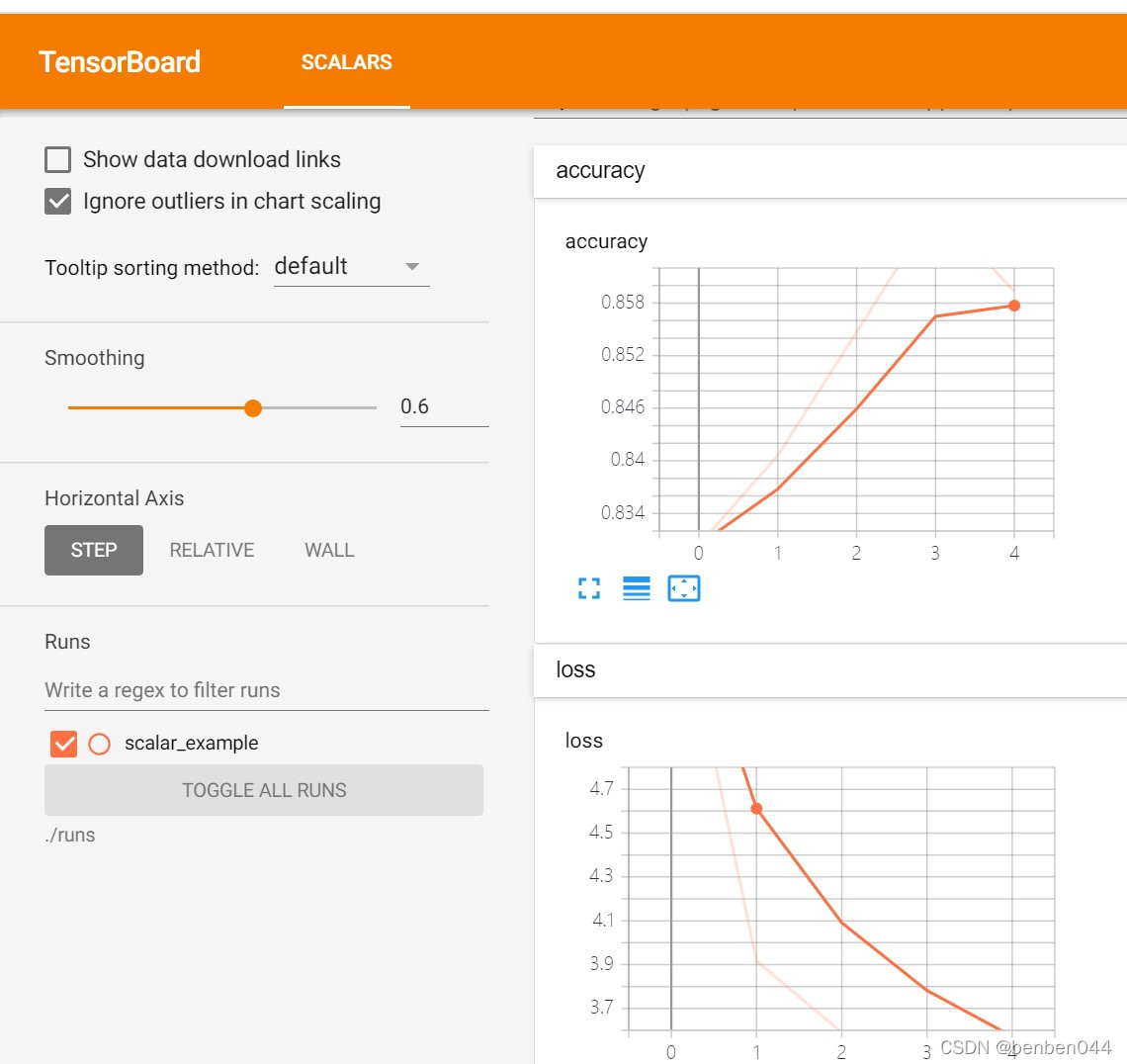
第9步，使用tensorboard跟踪训练结果

（1）安装tensorboard：

pip install tensorboardX

（2）在算法脚本下新建runs目录，后面tensorboard的日志都指定放到该目录之下

（3）日志插桩

from tensorboardX import SummaryWriter
writer = SummaryWriter('runs/scalar_example')

具体插桩示例如下：

loss_value = running_loss / print_every
accuracy_value = accuracy / (ii + 1)
print("Epoch: {}/{}".format(epoch + 1, epochs),
              "Loss: {:.4f}".format(loss_value),
              "Test accuracy: {:.4f}".format(accuracy_value))
writer.add_scalar("loss", loss_value, epoch)
writer.add_scalar("accuracy", accuracy_value, epoch)
running_loss = 0

（4）运行tensorboard：

在runs的上一级目录下运行如下程序：

tensorboard --logdir "./runs" --host=127.0.0.1

得到结果：