【SKNet】《Selective Kernel Networks》

CVPR-2019

caffe code： https://github.com/implus/SKNet/blob/master/models/sknet50.prototxt

caffe code 可视化工具： http://ethereon.github.io/netscope/#/editor

---

---

1 Background and Motivation

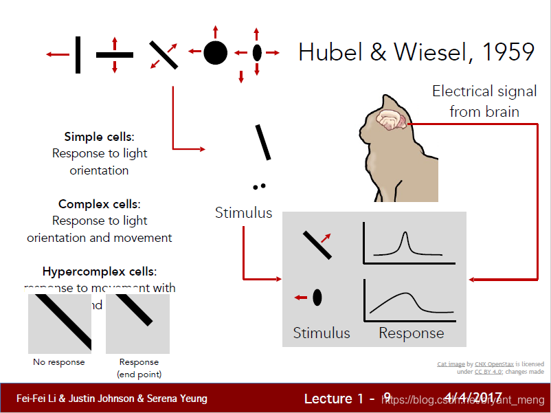
来自：cs231n课件链接

人类视皮质神经元的感受野是随着刺激的不同而变化的，然而 CNN 设计的时候，感受野是固定的！

It is well-known in the neuroscience community that the receptive field size of visual cortical neurons are modulated by the stimulus, which has been rarely considered in constructing CNNs.

Inception family 在这方面也做了尝试——同一stage，多个感受野 linear aggregation（the RF sizes of neurons in the same area (e.g., V1 region) are different），但还不能做到 adaptive changing of RF size.

【Inception-v1】《Going Deeper with Convolutions》（CVPR-2015）
【Inception-v2】《Batch Normalization: Accelerating Deep Network Training by Reducing Internal Covariate Shift》（ICML-2015）
【Inception-v3】《Rethinking the Inception Architecture for Computer Vision》（CVPR-2016）
【Inception-v4、Inception-Resnet-v1、v2】《Inception-v4, Inception-ResNet and the Impact of Residual Connections on Learning》（AAAI-2017）

作者想借鉴 visual cortical neurons 的特性，沿着 inception family 的发展线路，在 CNN 中做到 adaptive changing of receptive field（RF） size

2 Advantages / Contributions

提出了 SKNet，让 CNN 做到 adaptive changing of receptive field size！比 SENet 效果好！

3 Method

Split, Fuse and Select

adaptively change during inference

巧妙的 softmax 设计，666，很容易扩展到 multi-branch！

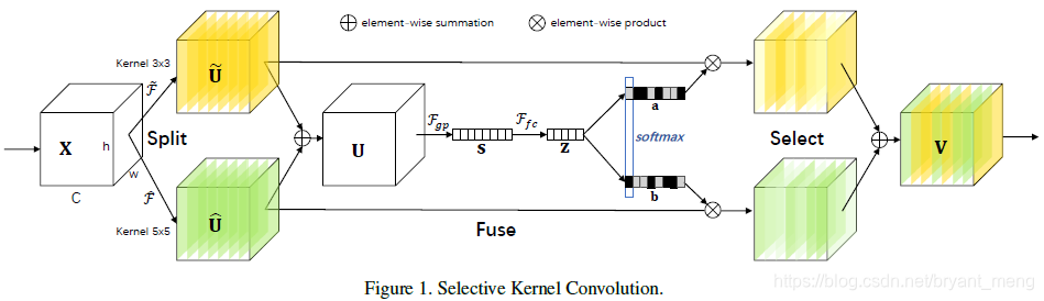
3.1 Selective Kernel Convolution

1）Split

特征图 $X\in {\mathbb{R}}^{H^{\prime }\times W^{\prime }\times C^{\prime }}$ 经过 3x3 和 5x5 卷积，生成特征图 $\tilde{U}\in {\mathbb{R}}^{H\times W\times C}$ 和 $\hat{U}\in {\mathbb{R}}^{H\times W\times C}$

为了减少计算量，conv 采用的是 grouped / depth-wise convolutions，5x5 用 3x3 配合 dilation 卷积来代替！

2）Fuse

做到 adaptive kernel，利用 gate 来实现

先 element-wise add

再 global average pooling 来做 channel wise 的 attention

接个 fc 来压缩下计算

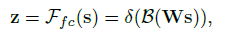
把向量 $s\in {\mathbb{R}}^{C\times 1}$ 压缩成 $z\in {\mathbb{R}}^{d\times 1}$，其中 $B$ 表示 batch normalization，$\delta$ 是 relu，$W\in {\mathbb{R}}^{d\times C}$ 表示权重！

压缩后的向量维度如下

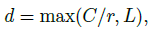
$L=32$，$r$ 是压缩比率！最低保留 32

3）Select

$z$ 经两个 fc 把向量恢复成通道数的一样的维度，接 softmax 激活

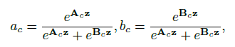
$z\in {\mathbb{R}}^{d\times 1}$，$A_c,B_c\in {\mathbb{R}}^{1\times d}$

$a，b\in {\mathbb{R}}^{C\times 1}$，

$a_c，b_c\in {\mathbb{R}}^{1\times 1}$，下标 $c$ 表示 $c$-th element

最后把 learning 到的 channel-wise attention 作用到原特征图上

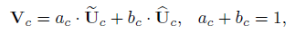
因为 two-branch 用的是 softmax，所以权重和为1，确实起到了 gate 的作用，控制两条分支的比重

$V\in {\mathbb{R}}^{H\times W\times C}$

3.2 Network Architecture

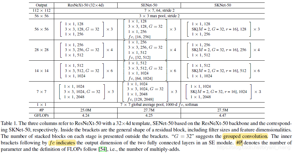
M 是 the number of paths，比如 fig 1 中 M = 2

第二列是在每个 bottleneck 结束后接一个 SK attention，第三列是在 bottleneck 内部使用，应该是在 3x3 conv 之后

4 Experiments

4.1 Datasets

• ImageNet 2012 dataset
• CIFAR-10
• CIFAR-100

4.2 ImageNet Classification

1）Comparisons with state-of-the-art models

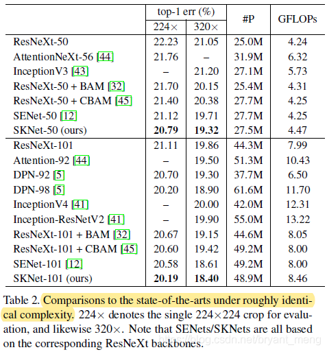
可以看到，SKNet-50 就表现出媲美其它 100 layer 的网络了

2）Selective Kernel vs. Depth/Width/Cardinality

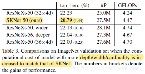
和 ResNeXt 皇城 PK，把参数量都调至相当的水平

3）Performance with respect to the number of parameters

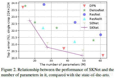
左下角最好，可以看到，SKNet utilizes parameters more efficiently than 其它的 models

4）Lightweight models

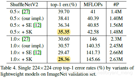
加在 shuffleNet 上有提升，且比 SE 的 channel attention 好

4.3 CIFAR Classification

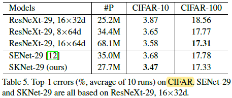
看 ResNeXt 的参数设置，分的组数不多，每组的 width 好大，32，64

SKNet 和 ResNeXt 相比，更少的参数量，更高的 acc

4.4 Ablation Studies

1）The dilation D and group number G

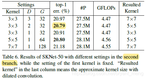
D 表示 dilation， G 是 group！难怪看 code 的时候，怎么两个 branch 都是 3x3，懵了半天，原来是配合 dilation convolution 是实现不同 kernel size 的！上面表展示了 second branch 的超参数调整实现

first branch 默认参数设定为，3x3 conv，D = 1，G = 32

作者发现，相同 RF 下，小的 kernel 配合 dilation 要比 大 kernel 好一丢丢（20.79 vs 20.78）

2）Combination of different kernels

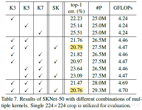
K3 是 3x3 conv，K5 是 3x3 配合 d = 2 的 dilation conv，K7 是 3x3 配合 d = 3 的 dilation conv

SK 的有无就是 fig1中 U 还是 V 的区别，也就是 branch 结合的时候，是线性的（U，element-wise addition）还是非线性的（V）

可以看到，M 越多效果越好，多个branch 的非线性组合（V）要比线性组合（U）结果好

M = 2 的时候 “性价比” 最高

4.5 Analysis and Interpretation

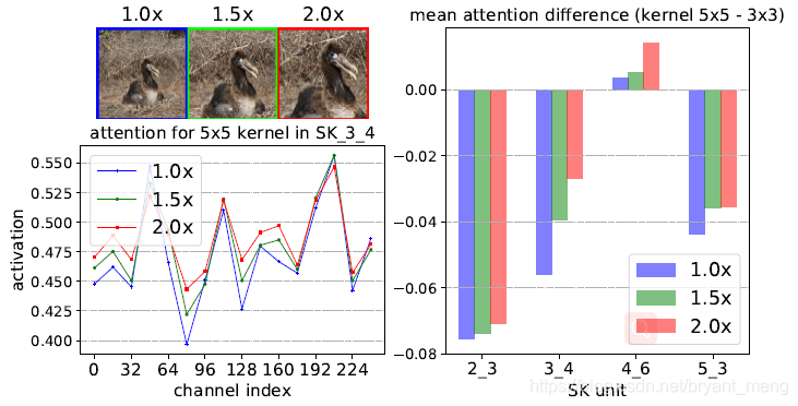
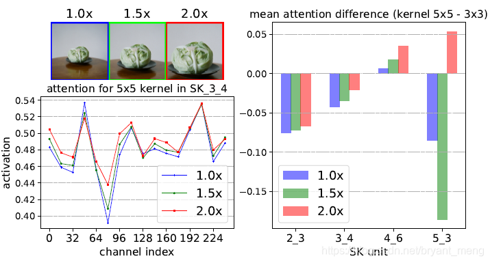
这两个图模式一样，

• 左上角是三种放大目标的原始图片
• 左下角是观察 SK_3_4 中 5x5 卷积的 attention 情况，横坐标是 channel 的索引，纵坐标是 channel-wise 的 weight，三条曲线对应三种原始图片！可以看到，随着目标的放大（1.0x to 2.0x），5x5 conv 的 weight 呈放大趋势
• 右边图是 SK unit 中，5x5 conv 的 channel-weight 减去 3x3 conv 的 channel-weight，可以看到，随着目标的放大（1.0x to 2.0x），5x5 conv 越来越重要，差值呈上升趋势！

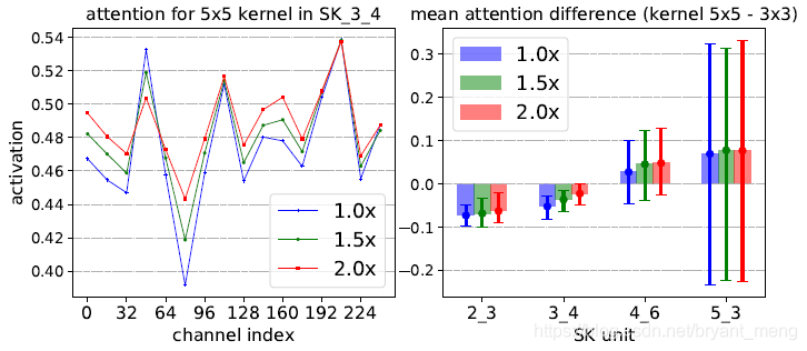
这个图是对所有例子（all image instances in the ImageNet validation set）的统计，大体结论和上面两个例子一样，就是目标越大，5x5 的 conv 的 attention weight 也越来越大，但随着 stage 的深入，这一规律消失

The larger the target object is, the more attention will be assigned to larger kernels by the Selective Kernel mechanism in low and middle level stages.(e.g., SK 2 3, SK 3 4).

在 high level 的 stage 中，这种现象消失了

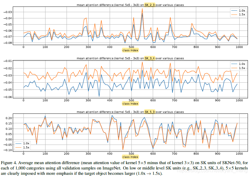
作者还探讨了类别上的效果，横坐标是类别索引（ 每类 50 个 sample），纵坐标是 5X5 和 3x3 两个 branch 的 channel-wise weight 的差值

可以看到，晚期的 stage 中，差距很小，早期和中期的 stage 差距明显，中期的差距最明显！！

作者对晚期 stage 差距不明显的解释如下：

since for the high-level representation, “scale” is partially encoded in the feature vector, and the kernel size matters less compared to the situation in lower layers.

就是说，high level 的 feature 本身就编码了 scale 信息，不太依赖不同的 kernel 来提取出了！

5 Conclusion（own）

• 是 inception 和 SENet 的巧妙结合
  inception 是设定的多个感受野线性聚合，SKNet 做到非线性的自适应的感受野大小

【Inception-v1】《Going Deeper with Convolutions》（CVPR-2015）
【SENet】《Squeeze-and-Excitation Networks》（CVPR-2018）

• inception family 的 motivation，the RF sizes of neurons in the same area (e.g., V1 region) are different, which enables the neurons to collect multi-scale spatial information in the same processing stage.

• related work 中 Multi-branch convolutional networks 还挺多论文的（Highway Network，resnet）

• 多种 kernel 可以配合 dilation 实现，666，这样还不用增加参数量！由于采用的是 softmax，作者的方法也很容易扩展到 multi-branch

• 注意作者对 high level 时，两种不同 kernel 的 attention weight 差距不明显的 解释！！！