


你将学会:
预处理图片数据
利用PaddlePaddle框架实现Logistic回归模型:
在开始练习之前,简单介绍一下图片处理的相关知识:
图片处理
由于识别猫问题涉及到图片处理知识,这里对计算机如何保存图片做一个简单的介绍。在计算机中,图片被存储为三个独立的矩阵,分别对应图中的红、绿、蓝三个颜色通道,如果图片是64*64像素的,就会有三个64*64大小的矩阵,要把这些像素值放进一个特征向量中,需要定义一个特征向量X,将三个颜色通道中的所有像素值都列出来。如果图片是64*64大小的,那么特征向量X的长度就是64*64*3,也就是12288。这样一个长度为12288的向量就是Logistic回归模型的一个训练数据。

目录
1 - 引用库
import sys
import numpy as np

import lr_utils
import matplotlib.pyplot as plt

import paddle
import paddle.fluid as fluid

from paddle.utils.plot import Ploter
%matplotlib inline
2 - 数据预处理
这里简单介绍数据集及其结构。数据集以hdf5文件的形式存储,包含了如下内容:
- 训练数据集:包含了m_train个图片的数据集,数据的标签(Label)分为cat(y=1)和non-cat(y=0)两类。
- 测试数据集:包含了m_test个图片的数据集,数据的标签(Label)同上。
单个图片数据的存储形式为(num_x, num_x, 3),其中num_x表示图片的长或宽(数据集图片的长和宽相同),数字3表示图片为三通道(RGB)。
需要注意的是,为了方便,添加“_orig”后缀表示该数据为原始数据,之后需要对数据做进一步处理。未添加“_orig”的数据则表示之后不需要再对该数据作进一步处理。
# 调用load_dataset()函数,读取数据集
train_set_x_orig, train_set_y, test_set_x_orig, test_set_y, classes = lr_utils.load_dataset()

# 图片示例
# 可观察到索引为“23”的图片应为“non-cat”
index = 19
plt.imshow(train_set_x_orig[index])
print ("y = " + str(train_set_y[:, index]) + ", it's a '" + classes[np.squeeze(train_set_y[:, index])].decode("utf-8") +  "' picture.")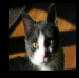
获取数据后的下一步工作是获得数据的相关信息,如训练样本个数 m_train、测试样本个数 m_test 和图片的长度或宽度 num_x,使用 numpy.array.shape 来获取数据的相关信息
m_train = train_set_x_orig.shape[0]
m_test = test_set_x_orig.shape[0]
num_px = train_set_x_orig.shape[1]


print ("训练样本数: m_train = " + str(m_train))
print ("测试样本数: m_test = " + str(m_test))
print ("图片高度/宽度: num_px = " + str(num_px))
print ("图片大小: (" + str(num_px) + ", " + str(num_px) + ", 3)")
print ("train_set_x shape: " + str(train_set_x_orig.shape))
print ("train_set_y shape: " + str(train_set_y.shape))
print ("test_set_x shape: " + str(test_set_x_orig.shape))
print ("test_set_y shape: " + str(test_set_y.shape))
训练样本数: m_train = 209 测试样本数: m_test = 50 图片高度/宽度: num_px = 64 图片大小: (64, 64, 3) train_set_x shape: (209, 64, 64, 3) train_set_y shape: (1, 209) test_set_x shape: (50, 64, 64, 3) test_set_y shape: (1, 50)
接下来需要对数据作进一步处理,为了便于训练,可以先忽略图片的结构信息,将包含图像长、宽和通道数信息的三维数组压缩成一维数组,图片数据的形状将由(64, 64, 3)转化为(64 * 64 * 3, 1)。
# 定义维度
DATA_DIM = num_px * num_px * 3

# 转换数据形状


train_set_x_flatten = train_set_x_orig.reshape(train_set_x_orig.shape[0], -1)
test_set_x_flatten = test_set_x_orig.reshape(test_set_x_orig.shape[0], -1)


print ("train_set_x_flatten shape: " + str(train_set_x_flatten.shape))
print ("train_set_y shape: " + str(train_set_y.shape))
print ("test_set_x_flatten shape: " + str(test_set_x_flatten.shape))
print ("test_set_y shape: " + str(test_set_y.shape))
在开始训练之前,还需要对数据进行归一化处理。图片采用红、绿、蓝三通道的方式来表示颜色,每个通道的单个像素点都存储着一个 0-255 的像素值,所以图片的归一化处理十分简单,只需要将数据集中的每个像素值除以 255 即可,但需要注意的是计算结果应为 float 类型。
train_set_x = train_set_x_flatten.astype('float32') / 255
test_set_x = test_set_x_flatten.astype('float32') / 255
为了方便后续的测试工作,添加了合并数据集和标签集的操作,使用 numpy.hstack 实现 numpy 数组的横向合并。
train_set = np.hstack((train_set_x, train_set_y.T))
test_set = np.hstack((test_set_x, test_set_y.T))
经过上面的实验,需要记住:
对数据进行预处理的一般步骤是:
- 了解数据的维度和形状等信息,例如(m_train, m_test, num_px, ...)
- 降低数据纬度,例如将数据维度(num_px, num_px, 3)转化为(num_px * num_px * 3, 1)
- 数据归一化
3 - 构造reader
构造read_data()函数,来读取训练数据集train_set或者测试数据集test_set。它的具体实现是在read_data()函数内部构造一个reader(),使用yield关键字来让reader()成为一个Generator(生成器),注意,yield关键字的作用和使用方法类似return关键字,不同之处在于yield关键字可以构造生成器(Generator)。虽然我们可以直接创建一个包含所有数据的列表,但是由于内存限制,我们不可能创建一个无限大的或者巨大的列表,并且很多时候在创建了一个百万数量级别的列表之后,我们却只需要用到开头的几个或几十个数据,这样造成了极大的浪费,而生成器的工作方式是在每次循环时计算下一个值,不断推算出后续的元素,不会创建完整的数据集列表,从而节约了内存使用。
# 读取训练数据或测试数据
def read_data(data_set):
    """
        一个reader
        Args:
            data_set -- 要获取的数据集
        Return:
            reader -- 用于获取训练数据集及其标签的生成器generator
    """
    def reader():
        """
        一个reader
        Args:
        Return:
            data[:-1], data[-1:] -- 使用yield返回生成器(generator),
            data[:-1]表示前n-1个元素组成的list,也就是训练数据,data[-1]表示最后一个元素,也就是对应的标签
        """
        for data in data_set:
            ### START CODE HERE ### (≈ 1 lines of code)
            yield data[:-1], data[-1]

            ### END CODE HERE ###
    return reader
test_array = [[1,1,1,1,0],
                [2,2,2,2,1],
                [3,3,3,3,0]]

print("test_array for read_data:")
for value in read_data(test_array)():
    print(value)


test_array for read_data:
([1, 1, 1, 1], 0)
([2, 2, 2, 2], 1)
([3, 3, 3, 3], 0)
4 - 训练过程
4.1 获取训练数据
关于参数的解释如下:
paddle.reader.shuffle(read_data(data_set), buf_size=BUF_SIZE)
 表示从read_data(data_set)这个reader中读取了BUF_SIZE大小的数据并打乱顺序

paddle.batch(reader(), batch_size=BATCH_SIZE)
 表示从reader()中取出BATCH_SIZE大小的数据进行一次迭代训练

BATCH_SIZE= 32

# 设置训练reader
train_reader = paddle.batch(
    paddle.reader.shuffle(
        read_data(train_set), buf_size=500),
    batch_size=BATCH_SIZE)

#设置测试 reader
test_reader = paddle.batch(
    paddle.reader.shuffle(
        read_data(test_set), buf_size=500),
    batch_size=BATCH_SIZE)
4.2配置网络结构和损失函数
Logistic 回归模型结构相当于一个只含一个神经元的神经网络,如下图所示,只包含输入数据以及输出层,不存在隐藏层,所以只需配置输入层(input)、输出层(predict)和标签层(label)即可。
#配置输入层、输出层、标签层
x = fluid.layers.data(name='x', shape=[DATA_DIM], dtype='float32')
y_predict = fluid.layers.fc(input=x, size=2, act='softmax')
y = fluid.layers.data(name='y', shape=[1], dtype='int64')


#定义损失函数
cost = fluid.layers.cross_entropy(input=y_predict, label=y)
avg_loss = fluid.layers.mean(cost)
acc = fluid.layers.accuracy(input=y_predict, label=y)
接下来,我们写三个语句分别来获取:
- ①全局主程序main program。该主程序用于训练模型。
- ②全局启动程序startup_program。该程序用于初始化。
- ③测试程序test_program。用于模型测试。
startup_program = fluid.default_startup_program()
main_program = fluid.default_main_program()

#克隆main_program得到test_program
#有些operator在训练和测试之间的操作是不同的,例如batch_norm,使用参数for_test来区分该程序是用来训练还是用来测试
#该api不会删除任何操作符,请在backward和optimization之前使用
test_program = fluid.default_main_program().clone(for_test=True)
4.3 设置优化方法
这里选择Adam优化算法:
optimizer = fluid.optimizer.Adam(learning_rate=0.001)
optimizer.minimize(avg_loss)
print("optimizer is ready")
4.4 定义训练场所
# 使用CPU训练
use_cuda = False
place = fluid.CUDAPlace(0) if use_cuda else fluid.CPUPlace()

#创建执行器和保存路径
exe = fluid.Executor(place)
save_dirname="recognize_cat_inference.model"

train_prompt = "Train cost"
cost_ploter = Ploter(train_prompt)

# 将训练过程绘图表示
def event_handler_plot(ploter_title, step, cost):
    cost_ploter.append(ploter_title, step, cost)
    cost_ploter.plot()
还可以定义一个train_test()函数,作用是:使用测试集数据,来测试训练效果。
def train_test(train_test_program, train_test_feed, train_test_reader):

     # 将分类准确率存储在acc_set中
    acc_set = []
    # 将平均损失存储在avg_loss_set中
    avg_loss_set = []

    # 将测试 reader yield 出的每一个数据传入网络中进行训练
    for test_data in train_test_reader():
        acc_np, avg_loss_np = exe.run(
            program=train_test_program,
            feed=train_test_feed.feed(test_data),
            fetch_list=[acc, avg_loss])
        acc_set.append(float(acc_np))
        avg_loss_set.append(float(avg_loss_np))

    # get test acc and loss
    # 获得测试数据上的准确率和损失值
    acc_val_mean = np.array(acc_set).mean()
    avg_loss_val_mean = np.array(avg_loss_set).mean()
    # 返回平均损失值,平均准确率
    return avg_loss_val_mean, acc_val_mean

feeder = fluid.DataFeeder(place=place, feed_list=[x, y])
exe.run(startup_program)
4.5设置训练主循环
构建一个循环来进行训练,直至训练完成,把模型保存到 params_dirname 。
exe.run(fluid.default_startup_program())

PASS_NUM = 150
epochs = [epoch_id for epoch_id in range(PASS_NUM)]


lists = []

step = 0
for epoch_id in epochs:
    for step_id, data in enumerate(train_reader()):
        metrics = exe.run(
            main_program,
            feed=feeder.feed(data),
            fetch_list=[avg_loss,acc])
        #我们可以把训练结果打印输出,也可以用画图展示出来
        if step % 10 == 0: #每训练10次,绘制一次曲线
            event_handler_plot(train_prompt, step, metrics[0])
        step += 1

    # 测试每个epoch的分类效果
    avg_loss_val, acc_val = train_test(
        train_test_program=test_program,
        train_test_reader=test_reader,
        train_test_feed=feeder)

    print("Test with Epoch %d, avg_cost: %s, acc: %s" %
          (epoch_id, avg_loss_val, acc_val))
    lists.append((epoch_id, avg_loss_val, acc_val))

# 保存训练好的模型参数用于预测
if save_dirname is not None:
    fluid.io.save_inference_model(save_dirname, ["x"], [y_predict], exe)

# 选择效果最好的pass
best = sorted(lists, key=lambda list: float(list[1]))[0]
print('Best pass is %s, testing Avgcost is %s' % (best[0], best[1]))
print('The classification accuracy is %.2f%%' % (float(best[2]) * 100))

5 - 预测阶段
#指定预测的作用域
inference_scope = fluid.core.Scope()
with fluid.scope_guard(inference_scope):

    # 使用 fluid.io.load_inference_model 获取 inference program,
    # feed_target_names 用于指定需要传入网络的变量名
    # fetch_targets 指定希望从网络中fetch出的变量名
    [inference_program, feed_target_names,
     fetch_targets] = fluid.io.load_inference_model(
         save_dirname, exe)

    # 将feed构建成字典 {feed_target_name: feed_target_data}
    # 结果将包含一个与fetch_targets对应的数据列表
    # 我们可以实现批量预测,通过一个循环,每次预测一个mini_batch
    for mini_batch in test_reader():
        test_x = np.array([data[0] for data in mini_batch]).astype("float32")
        test_y = np.array([data[1] for data in mini_batch]).astype("int64")
        # 真实进行预测
        mini_batch_result = exe.run(
            inference_program,
            feed={feed_target_names[0]: test_x},
            fetch_list=fetch_targets)

        # 打印预测结果
        mini_batch_result = np.argsort(mini_batch_result) #找出可能性最大的列标,升序排列
        mini_batch_result = mini_batch_result[0][:, -1]  #把这些列标拿出来
        print('预测结果:%s'%mini_batch_result)

        # 打印真实结果
        label = test_y # 转化为 label
        print('真实结果:%s'%label)

    #计数
    label_len = len(label)
    right_counter = 0
    for i in range(label_len):
        if mini_batch_result[i] == label[i]:
            right_counter += 1

    ratio = (right_counter/label_len)
    print("准确率为:%.2f%%"%(ratio*100))
预测结果:[1 0 1 0 0 1 0 0 1 0 0 0 0 1 0 0 1 1 1 1 0 0 1 1 0 1 0 1 1 1 1 0] 真实结果:[0 1 1 1 0 1 1 0 0 0 0 1 0 1 0 1 1 1 1 0 1 0 1 1 1 0 1 1 1 1 1 0] 预测结果:[0 0 0 1 1 1 1 0 1 1 1 1 0 1 1 0 1 1] 真实结果:[1 1 0 1 1 0 1 0 1 1 1 1 0 1 1 0 1 1] 准确率为:83.33%
6 - 总结
通过这个练习应该记住:
至此Logistic回归模型的训练工作完成,在使用PaddlePaddle进行模型配置和训练的过程中不用考虑参数的初始化、成本函数、激活函数、梯度下降、参数更新和预测等具体细节;只需要简单地配置网络结构和trainer即可,并且PaddlePaddle提供了许多接口来改变学习率、成本函数、批次大小等许多参数来改变模型的学习效果,使用起来更加灵活,方便测试,在之后的练习中,会对PaddlePaddle更加熟悉。


 1898
1898


 被折叠的 条评论
为什么被折叠?
被折叠的 条评论
为什么被折叠?
 到【灌水乐园】发言


