


欢迎关注更多精彩
关注我,学习常用算法与数据结构,一题多解,降维打击。
本期话题:最小二乘圆柱拟合
相关背景资料
点击前往

圆柱拟合输入和输出要求
输入
- 8到50个点,全部采样自圆柱上。
- 每个点3个坐标,坐标精确到小数点后面20位。
- 坐标单位是mm, 范围[-500mm, 500mm]。
tips
输入虽然是严格来自圆柱,但是由于浮点表示,记录的值和真实值始终是有微小的误差,点云到拟合圆柱的距离不可能完全为0。
输出
- 1点X0表示 圆柱中心轴上1点,用三个坐标表示。
- 法向A代表圆柱中心轴法向。
- 圆半径r。
精度要求
- X0点到标准圆柱中心轴距离不能超过0.0001mm。
- 法向A与圆柱法向夹角不能超过0.0000001rad。
- r与标准半径的差不能超过0.0001mm。
圆柱优化标函数
根据论文,圆柱拟合转化成数学表示如下:
圆柱参数化表示
- 圆柱中心轴上1点X0 = (x0, y0, z0)。
- 法向A=(a,b,c)。
- 半径r。
圆柱方程 u 2 + v 2 + w 2 a 2 + b 2 + c 2 = r 2 u i = c ( y − y 0 ) − b ( z − z 0 ) v i = a ( z − z 0 ) − c ( x − x 0 ) w i = b ( x − x 0 ) − a ( y − y 0 ) 圆柱方程\begin {array}{l}\frac {u^2+v^2+w^2} {a^2+b^2+c^2}=r^2 \\ u_i =c(y-y_0)-b(z-z_0)\\ v_i=a(z-z_0)-c(x-x_0)\\ w_i=b(x-x_0)-a(y-y_0)\ \end {array} 圆柱方程a2+b2+c2u2+v2+w2=r2ui=c(y−y0)−b(z−z0)vi=a(z−z0)−c(x−x0)wi=b(x−x0)−a(y−y0)
能量方程
第i个点 pi(xi, yi, zi)。
距离函数
d i = r i − r d_i = r_i-r di=ri−r
r i = u 2 + v 2 + w 2 u i = c ( y − y 0 ) − b ( z − z 0 ) v i = a ( z − z 0 ) − c ( x − x 0 ) w i = b ( x − x 0 ) − a ( y − y 0 ) \begin {array}{l}r_i = \sqrt{u^2+v^2+w^2} \\ u_i =c(y-y_0)-b(z-z_0)\\ v_i=a(z-z_0)-c(x-x_0)\\ w_i=b(x-x_0)-a(y-y_0) \end {array} ri=u2+v2+w2ui=c(y−y0)−b(z−z0)vi=a(z−z0)−c(x−x0)wi=b(x−x0)−a(y−y0)
根据定义得到能量方程
E = ∑ 1 n d i 2 E=\displaystyle \sum _1^n {d_i^2} E=1∑ndi2
最小二乘优化能量方程
能量方程 E = f ( X 0 , A , r ) = ∑ 1 n d i 2 E=f(X0, A, r)=\displaystyle \sum _1^n {d_i^2} E=f(X0,A,r)=1∑ndi2
上式是一个7元二次函数中,X0, A, r是未知量,拟合圆柱的过程也可以理解为优化X0, A, r使得方程E最小。
上述方程直接求导不好解,可以使用高斯牛顿迭代法。
高斯牛顿迭代法
用于解非线性最小二乘问题。同时,高斯牛顿法需要比较可靠的初值,所以寻找目标函数的初值也是一个比较关键的步骤。
基本原理
设 a = ( a 0 , a 1 , . . . , a n ) 是待求解向量, a ^ 是初始给定值, a = a ^ + Δ a , Δ a 是我们每次迭代后移动的量 设 a=(a_0, a_1,...,a_n)是待求解向量,\widehat {a} 是初始给定值,a = \widehat {a} +\Delta a, \Delta a 是我们每次迭代后移动的量 设a=(a0,a1,...,an)是待求解向量,a 是初始给定值,a=a +Δa,Δa是我们每次迭代后移动的量
定义距离函数为 F ( x , a ) , d i = F ( x i , a ) , 进行泰勒 1 阶展开, F ( x , a ) = F ( x , a ^ ) + ∂ F ∂ a ^ Δ a = F ( x , a ^ ) + J Δ a 定义距离函数为 F(x, a), d_i = F(x_i, a), 进行泰勒1阶展开, F(x, a) = F(x, \widehat a) + \frac {\partial F}{\partial \widehat a}\Delta a = F(x, \widehat a) + J\Delta a 定义距离函数为F(x,a),di=F(xi,a),进行泰勒1阶展开,F(x,a)=F(x,a )+∂a ∂FΔa=F(x,a )+JΔa
每次迭代,其实就是希望通过调整 Δ a 使得 J Δ a = − F ( x , a ^ ) 每次迭代,其实就是希望通过调整\Delta a 使得 J\Delta a = -F(x, \widehat a) 每次迭代,其实就是希望通过调整Δa使得JΔa=−F(x,a )
J = [ ∂ F ( x 0 , a ) ∂ a 0 ∂ F ( x 0 , a ) ∂ a 1 . . . ∂ F ( x 0 , a ) ∂ a n ∂ F ( x 1 , a ) ∂ a 0 ∂ F ( x 1 , a ) ∂ a 1 . . . ∂ F ( x 1 , a ) ∂ a n . . . . . . . . . . . . ∂ F ( x n , a ) ∂ a 0 ∂ F ( x n , a ) ∂ a 1 . . . ∂ F ( x n , a ) ∂ a n ] J = \begin {bmatrix} \frac {\partial F(x_0, a)} {\partial a_0} & \frac {\partial F(x_0, a)} {\partial a_1} & ...& \frac {\partial F(x_0, a)} {\partial a_n} \\ \\ \frac {\partial F(x_1, a)} {\partial a_0} & \frac {\partial F(x_1, a)} {\partial a_1} & ...& \frac {\partial F(x_1, a)} {\partial a_n} \\\\ ... & ... & ...& ... \\ \\ \frac {\partial F(x_n, a)} {\partial a_0} & \frac {\partial F(x_n, a)} {\partial a_1} & ...& \frac {\partial F(x_n, a)} {\partial a_n} \end {bmatrix} J= ∂a0∂F(x0,a)∂a0∂F(x1,a)...∂a0∂F(xn,a)∂a1∂F(x0,a)∂a1∂F(x1,a)...∂a1∂F(xn,a)............∂an∂F(x0,a)∂an∂F(x1,a)...∂an∂F(xn,a)
F ( x , a ^ ) = [ d 1 d 2 . . . d m ] F(x, \widehat a) = \begin {bmatrix} d_1 \\ d_2 \\... \\ d_m \end {bmatrix} F(x,a )= d1d2...dm
J Δ a = − F ( x , a ^ ) , 解出 Δ a , 更新 a = a ^ + Δ a , 持续迭代直到 Δ a 足够小 J\Delta a = -F(x,\widehat a), 解出\Delta a ,更新 a = \widehat {a} +\Delta a, 持续迭代直到\Delta a足够小 JΔa=−F(x,a ),解出Δa,更新a=a +Δa,持续迭代直到Δa足够小
用4个数表示直线法向
如果直接拿6个参数表示直线去做迭代,1是比较麻烦,会出现比较难解的方向,2是法向长度不固定,结果不唯一。
当直线与Z轴偏差比较小的时候可以使用4个参数来表示直线。
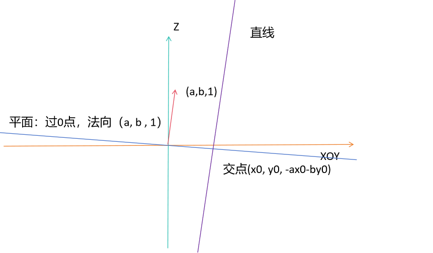
如上图,绿线为Z轴,橙色线为XOY平面。
由于法向与Z轴比较相近,可以设法向为(a, b, 1), a,b 是比较小的量。
规定直线上1点需要在以(a, b, 1)为法向,过0点的平面上。
则有 ax0+by0 + z0=0, 只要知道x0, y0 可知 z0 = -ax0-by0。
模型简化
为了使用上述方法,当得到一个拟合初值后,需要先将中心线旋转致Z轴,把圆心移致0点。
此时,
x0=y0=z0=0.
a=b=0, c=1.
r i = ( x i 2 + y i 2 ) \begin {array}{l}r_i=\sqrt{(x_i^2+y_i^2)}\end {array} ri=(xi2+yi2)
算法描述
我们希望di0。
可以对di分别求偏导
J, D的计算。
J = ∂ d 1 ∂ x 0 ∂ d 1 ∂ y 0 ∂ d 1 ∂ a ∂ d 1 ∂ b ∂ d 1 ∂ r ∂ d 2 ∂ x 0 ∂ d 2 ∂ y 0 ∂ d 2 ∂ a ∂ d 2 ∂ b ∂ d 2 ∂ r . . . . . . . . . . . . . . . ∂ d n ∂ x 0 ∂ d n ∂ y 0 ∂ d n ∂ a ∂ d n ∂ b ∂ d n ∂ r , D = d 1 d 2 . . . d n J= \begin{array}{l} \frac {\partial d_1}{\partial x_0}& \frac {\partial d_1}{\partial y_0}& \frac {\partial d_1}{\partial a}& \frac {\partial d_1}{\partial b}& \frac {\partial d_1}{\partial r} \\ \frac {\partial d_2}{\partial x_0}& \frac {\partial d_2}{\partial y_0}& \frac {\partial d_2}{\partial a}& \frac {\partial d_2}{\partial b}& \frac {\partial d_2}{\partial r}\\...&...&...&...&...\\\frac {\partial d_n}{\partial x_0}& \frac {\partial d_n}{\partial y_0}& \frac {\partial d_n}{\partial a}& \frac {\partial d_n}{\partial b}& \frac {\partial d_n}{\partial r}\\ \end {array}, \ D= \begin{array}{l} d_1\\d_2\\...\\d_n\end {array} J=∂x0∂d1∂x0∂d2...∂x0∂dn∂y0∂d1∂y0∂d2...∂y0∂dn∂a∂d1∂a∂d2...∂a∂dn∂b∂d1∂b∂d2...∂b∂dn∂r∂d1∂r∂d2...∂r∂dn, D=d1d2...dn
5个未知分别对d_i求导结果如下:
回顾一下
u i = c ( y i − y 0 ) − b ( z i − z 0 ) v i = a ( z i − z 0 ) − c ( x i − x 0 ) w i = b ( x i − x 0 ) − a ( y i − y 0 ) \begin {array}{l}u_i =c(y_i-y_0)-b(z_i-z_0)\\ v_i=a(z_i-z_0)-c(x_i-x_0)\\ w_i=b(x_i-x_0)-a(y_i-y_0)\end {array} ui=c(yi−y0)−b(zi−z0)vi=a(zi−z0)−c(xi−x0)wi=b(xi−x0)−a(yi−y0)
∂ d i ∂ x 0 = u i 2 + v i 2 + w i 2 − r ∂ x 0 = ( x i − x 0 ) 2 ∂ x 0 2 u i 2 + v i 2 + w i 2 = − x i x i 2 + y i 2 \frac {\partial d_i} {\partial x_0}=\frac {\sqrt{u_i^2+v_i^2+w_i^2}-r} {\partial x_0} \\ =\frac {\frac {(x_i-x_0)^2}{\partial x_0}}{2\sqrt{u_i^2+v_i^2+w_i^2}}\\ =\frac {-x_i}{\sqrt{x_i^2+y_i^2}} ∂x0∂di=∂x0ui2+vi2+wi2−r=2ui2+vi2+wi2∂x0(xi−x0)2=xi2+yi2−xi
∂ d i ∂ y 0 = u i 2 + v i 2 + w i 2 − r ∂ y 0 = ( y i − y 0 ) 2 ∂ y 0 2 u i 2 + v i 2 + w i 2 = − y i x i 2 + y i 2 \frac {\partial d_i} {\partial y_0}=\frac {\sqrt{u_i^2+v_i^2+w_i^2}-r} {\partial y_0} \\ =\frac {\frac {(y_i-y_0)^2}{\partial y_0}}{2\sqrt{u_i^2+v_i^2+w_i^2}}\\ =\frac {-y_i}{\sqrt{x_i^2+y_i^2}} ∂y0∂di=∂y0ui2+vi2+wi2−r=2ui2+vi2+wi2∂y0(yi−y0)2=xi2+yi2−yi
∂ d i ∂ a = u i 2 + v i 2 + w i 2 − r ∂ a = [ a ( z i − z 0 ) − c ( x i − x 0 ) ] 2 ∂ a 2 u i 2 + v i 2 + w i 2 = − x i z i x i 2 + y i 2 \frac {\partial d_i} {\partial a}=\frac {\sqrt{u_i^2+v_i^2+w_i^2}-r} {\partial a}\\ =\frac {\frac {[a(z_i-z_0)-c(x_i-x_0)]^2}{\partial a}}{2\sqrt{u_i^2+v_i^2+w_i^2}}\\ =\frac {-x_iz_i}{\sqrt{x_i^2+y_i^2}} ∂a∂di=∂aui2+vi2+wi2−r=2ui2+vi2+wi2∂a[a(zi−z0)−c(xi−x0)]2=xi2+yi2−xizi
∂ d i ∂ b = u i 2 + v i 2 + w i 2 − r ∂ b = [ c ( y i − y 0 ) − b ( z i − z 0 ) ] 2 ∂ b 2 u i 2 + v i 2 + w i 2 = − y i z i x i 2 + y i 2 \frac {\partial d_i} {\partial b}=\frac {\sqrt{u_i^2+v_i^2+w_i^2}-r} {\partial b}\\ =\frac {\frac {[c(y_i-y_0)-b(z_i-z_0)]^2}{\partial b}}{2\sqrt{u_i^2+v_i^2+w_i^2}}\\ =\frac {-y_iz_i}{\sqrt{x_i^2+y_i^2}} ∂b∂di=∂bui2+vi2+wi2−r=2ui2+vi2+wi2∂b[c(yi−y0)−b(zi−z0)]2=xi2+yi2−yizi
∂ d i ∂ r = u i 2 + v i 2 + w i 2 − r ∂ r = − 1 \frac {\partial d_i} {\partial r}=\frac {\sqrt{u_i^2+v_i^2+w_i^2}-r} {\partial r} = -1 ∂r∂di=∂rui2+vi2+wi2−r=−1
-
确定圆初值
-
将中轴通过刚体变换U至Z轴,U的构建可以参考代码
[ x i y i z i ] = U ⋅ ( [ x i y i z i ] − [ x 0 y 0 z 0 ] ) \begin {bmatrix}x_i \\ y_i \\ z_i \end {bmatrix} = U \cdot \left (\begin {bmatrix}x_i \\ y_i \\ z_i \end {bmatrix}- \begin{bmatrix}x_0 \\ y_0 \\ z_0 \end {bmatrix}\right ) xiyizi =U⋅ xiyizi − x0y0z0 -
根据上述公式构建 J ⋅ ( [ p x 0 p y 0 p a p b p r ] ) = − D J \cdot \left(\begin {bmatrix}p_{x_0} \\ p_{y_0}\\p_a\\p_b\\p_{r} \end {bmatrix} \right)=-D J⋅ px0py0papbpr =−D
-
求解 Δ p \Delta p Δp
-
更新解
[ x 0 y 0 z 0 ] = [ x 0 y 0 z 0 ] + U T ⋅ [ p x 0 p y 0 − p a p x 0 − p b p y 0 ] [ a b c ] = U T ⋅ [ p a p b 1 ] . n o r m a l i z e ( ) r = r + p r \begin {array}{l}\\ \begin {bmatrix}x_0 \\ y_0 \\ z_0 \end {bmatrix} = \begin {bmatrix}x_0 \\ y_0 \\ z_0 \end {bmatrix} + U^T \cdot \begin{bmatrix}p_{x_0} \\ p_{y_0}\\ -p_ap_{x_0}-p_bp_{y_0}\end {bmatrix} \\ \\\begin {bmatrix}a \\ b \\ c \end {bmatrix} = U^T \cdot \begin{bmatrix}p_a \\ p_b \\ 1 \end {bmatrix}.normalize() \\\\ r=r+p_r \end {array} x0y0z0 = x0y0z0 +UT⋅ px0py0−papx0−pbpy0 abc =UT⋅ papb1 .normalize()r=r+pr -
重复2直到收敛
初值确定
可以枚举法向(间隔1度),把所有点投影到该法向的任意平面上,求出平面上的圆。以误差最小的圆作为半径,圆心作为中轴上一点。可以并行加速。
代码实现
代码链接:https://gitcode.com/chenbb1989/3DAlgorithm/tree/master/CBB3DAlgorithm/Fitting
#include "CylinderFitter.h"
#include "CircleFitter.h"
#include <corecrt_math_defines.h>
#include <Eigen/Dense>
#include<iostream>


namespace Gauss {
	double F(Fitting::Cylinder cylinder, const Point& p)
	{
		double di = (p - cylinder.center).cross(cylinder.orient).norm() - cylinder.r;
		return di;
	}
	double GetError(Fitting::Cylinder cylinder, const std::vector<Eigen::Vector3d>& points)
	{
		double err = 0;
		for (auto& p : points) {
			double d = F(cylinder, p);
			err += d * d;
		}
		err /= points.size();
		return err;
	}
	Fitting::Matrix CylinderFitter::Jacobi(const std::vector<Eigen::Vector3d>& points)
	{
		int n = points.size();
		Fitting::Matrix J(n, 5);
		for (int i = 0; i < n; ++i) {
			auto& p = points[i];
			double ri = Eigen::Vector2d(p.x(), p.y()).norm();

			//di求导
			J(i, 0) = -p.x() / ri;
			J(i, 1) = -p.y() / ri;
			J(i, 2) = -p.x() * p.z() / ri;
			J(i, 3) = -p.y() * p.z() / ri;
			J(i, 4) = -1;
		}
		return J;
	}

	void CylinderFitter::beforHook(const std::vector<Eigen::Vector3d>& points)
	{
		U = Fitting::getRotationByOrient(cylinder.orient);
		for (int i = 0; i < points.size(); ++i) {
			transPoints[i] = U * (points[i] - cylinder.center);
		}
	}
	void CylinderFitter::afterHook(const Eigen::VectorXd& xp)
	{
		cylinder.center += U.transpose() * Eigen::Vector3d(xp(0), xp(1), -xp(2)*xp(0)-xp(3)*xp(1));
		cylinder.orient = U.transpose() * Eigen::Vector3d(xp(2), xp(3), 1).normalized();
		cylinder.r += xp(4);
	}
	Eigen::VectorXd CylinderFitter::getDArray(const std::vector<Eigen::Vector3d>& points)
	{
		int n = points.size();
		Eigen::VectorXd D(points.size());
		for (int i = 0; i < points.size(); ++i) D(i) = Eigen::Vector2d(points[i].x(), points[i].y()).norm() - cylinder.r;
		return D;
	}
	bool CylinderFitter::GetInitFit(const std::vector<Eigen::Vector3d>& points)
	{
		if (points.size() < 5)return false;
		double cylinerErr = -1;
		transPoints.resize(points.size());
		Point center = Fitting::getCenter(points);
		// 拟合平面
		Fitting::FittingBase* fb = new CircleFitter();
		Fitting::Circle cir;
		int cnt = 0;
		for (double i = 0; i < 180; ++i) {
			double theta = i / 180 * M_PI;
			for (double j = 0; j < 180; ++j) {
				double alpha = j / 180 * M_PI;
				Point orient(cos(theta) , sin(theta)*cos(alpha),sin(theta)*sin(alpha));
				// 投影平面
				for (int k = 0; k < points.size(); ++k) {
					double d = (center-points[k]).dot(orient);
					transPoints[k] = points[k] + d * orient;
				}

				// 拟合圆
				double err = fb->Fitting(transPoints, &cir);
				if (err>0 && (cylinerErr < 0 || err < cylinerErr)) {
					//std::cout << "error : "<< err << std::endl;
					cylinerErr = err;
					cylinder.center = cir.center;
					cylinder.orient = cir.orient;
					cylinder.r = cir.r;
				}
				//cnt++;
				//if(cnt%100==0) std::cout << cnt << std::endl;

			}
			if (cylinerErr < 1e-4)break;
		}
		delete fb;
		return true;
	}
	double CylinderFitter::F(const Eigen::Vector3d& p)
	{
		return Gauss::F(cylinder, p);
	}
	double CylinderFitter::GetError(const std::vector<Eigen::Vector3d>& points)
	{
		return Gauss::GetError(cylinder, points);
	}
	void CylinderFitter::Copy(void* ele)
	{
		memcpy(ele, &cylinder, sizeof(Fitting::Cylinder));
	}
}
测试代码
#include "TestCylinder.h"
#include "CylinderFitter.h"
#include <iostream>

namespace Gauss {

	double TestCylinder::Fitting() {
		Fitting::FittingBase* fb = new Gauss::CylinderFitter();
		auto err = fb->Fitting(points, &fitResult);
		return err;
	}
	bool TestCylinder::JudgeAnswer(FILE* fp) {
		ReadAnswer();
		if (!lineCmp(ans.orient, ans.center, fitResult.center))return false;
		if (!orientationCmp(ans.orient, fitResult.orient))return false;
		if (!radiusCmp(ans.r, fitResult.r))return false;
		return true;
	}
	void TestCylinder::ReadAnswer() {
		vector<double> nums;
		if (PointCloud::readNums((suffixName + "/answer/" + fileName + ".txt"), nums)) {
			for (int i = 0; i < 3; ++i) ans.center[i] = nums[i];
			for (int i = 0; i < 3; ++i) ans.orient[i] = nums[i+3];
			ans.r = nums[6];
		}
		else {
			std::cout << "read answer error" << std::endl;
		}
	}
	void TestCylinder::SaveAnswer(FILE* fp) {
		writePoint(fp, fitResult.center);
		writePoint(fp, fitResult.orient);
		writeNumber(fp, fitResult.r);
	}
}
测试结果
https://gitcode.com/chenbb1989/3DAlgorithm/blob/master/CBB3DAlgorithm/Fitting/gauss/fitting_result/result.txt

b16 : CYLINDER : pass
b17 : CYLINDER : pass
b18 : CYLINDER : pass
b19 : CYLINDER : pass
b20 : CYLINDER : pass
b21 : CYLINDER : pass
b22 : CYLINDER : pass
b23 : CYLINDER : pass
b24 : CYLINDER : pass
b25 : CYLINDER : pass
本人码农,希望通过自己的分享,让大家更容易学懂计算机知识。创作不易,帮忙点击公众号的链接。


 1315
1315


 被折叠的 条评论
为什么被折叠?
被折叠的 条评论
为什么被折叠?
 到【灌水乐园】发言


