神经网络与深度学习-1- 机器学习概述-PyTorch

最新推荐文章于 2024-01-22 20:38:30 发布

明朝百晓生

最新推荐文章于 2024-01-22 20:38:30 发布

阅读量1k

点赞数

分类专栏：人工智能文章标签：深度学习机器学习神经网络

4AM_明朝百晓生

本文链接：https://blog.csdn.net/chengxf2/article/details/124407822

版权

人工智能专栏收录该内容

102 篇文章 3 订阅

订阅专栏

前言：

《神经网络与深度学习》邱锡鹏

https://www.bilibili.com/video/BV1Vx411j7kT?spm_id_from=333.337.search-card.all.click
https://www.bilibili.com/video/BV1Sr4y1N71H?spm_id_from=333.337.search-card.all.click
https://www.bilibili.com/video/BV1244y1G7B8?spm_id_from=333.337.search-card.all.click
https://www.bilibili.com/video/BV1uZ4y1C7gU?spm_id_from=333.337.search-card.all.click

毕业以后一直从事于通讯行业，接触学习机器学习和图像大概有4年左右，

回头看，对现在了解通讯更深层次的一些算法原理非常有帮助

基本概念
机器学习三要素
模型
学习准则
优化算法
线性回归例子

一基本概念

Feature: 基本特征，通常用列向量表示 $x=\begin{bmatrix} x_1 & x_2 & ... & x_n \end{bmatrix}^T$

Label: 标签，通常用y 表示

sample: 样本 D

Data Set: 数据集

Training Set: 训练集

Test Set: 测试数据集

给定训练集D，我们希望让计算机从一个函数集合

$F=\begin{Bmatrix} f_1(x) & f_2(x) & , & .... \end{Bmatrix}$

中寻找一个最优的函数 $f^{*}(x)$ ,来近似每个样本的特征向量x 和标签值之间的真实映射关系

对于一个样本x，我们可以通过 $f^{*}(x)$ 来预测其标签值

$\hat{y}=f^{*}(x)$

如何寻找这个最优的函数 $f^{*}(x)$ 是关键

一般都要通过学习算法（Learing Algorithm）来完成

这个寻找最优函数的过程称为学习或者train

二机器学习三要素

模型,学习准则,优化算法。后面跟人讨论也可以基于这三方面,加上一个应用场景。

三模型

机器学习任务，首先要确认输入空间X和输出空间Y

映射函数系数，网络结构图

首先我们不知道隐射函数g(x) 和条件概率分布 $P_r(y|x)$ 的具体形式

因此只能根据假设检验来假设一个函数集合F,称为假设空间（Hypothesis Space）

然后通过观测其在训练集D上的特性，从中选择一个理想的假设 $f^{*} \in F$

假设空间通常为一个参数化的函数族：

$F=\begin{Bmatrix} f(x;\theta)|\theta \in R^D \end{Bmatrix}$

其中 $f(x;\theta)$ 是参数 $\theta$ 的模型，D为参数的维度

常见的假设空间可以分为：

线性,非线性

四学习准则

4.1：损失函数

设训练集 $D=\begin{Bmatrix} x^n,y^n \end{Bmatrix}_{n=1}^{N}$ 由N个独立同分布的样本组成（IID: Independent and Identically Distributed ）

一个好的模型 $f(x,\theta^*)$ 应该在所有的样本空间上与真实的标签值一致

$|f(x,\theta^*)-y|<\epsilon$

或与真实条件概率 $P_r(y|x)$ 一致，即

$|f_y(x,\theta^*)-P_r(y|x)|<\epsilon$

模型的好坏可以通过（Expected Risk）期望风险来衡量

$R(\theta)=E_{(x,y)\sim P_r(x,y)}[L(y,f(x,\theta))]$

2.3 损失函数
常见四种：

0-1 损失函数：

$L(f(x,\theta),y)=\left\{\begin{matrix} 0, if y=f(x;\theta)\\ 1 ,if y \neq f(x;\theta) \end{matrix}\right. = I(y \neq f(x,\theta))$

优点：

能客观评价模型好坏

缺点：

导数为0，难以优化

平均损失函数(Quadratic Loss Function)：

$L(y,f(x;\theta))=\frac{1}{2}(y-f(x;\theta))^2$

适用于标签值为连续型数据

数理统计中矩估计的应用

交叉熵损失函数（Cross-Entropy Loss Function）

$L=-y^Tlogf(x;\theta)$

$=\sum_{c=1}^Cy_c log f_c(x;\theta)$

y 经常用one-hot 编码，例如一个三分类问题：

$y=[0,0,1],f(x;\theta)=[0.3,0.3,0.4]^T$ $L=-(0*log0.3+0*log0.3+1*log0.4)=-log0.4$

对于二分类问题,假设 $y \in \begin{Bmatrix} -1,+1 \end{Bmatrix}$ ， $f(x;\theta) \in R$

Hinge 损失函数为： $L(y,f(x;\theta))=max(0,1-yf(x;\theta))$

2：风险最小化准则

期望风险

针对所有的数据集 , 期望风险是模型关于联合分布的期望损失

我们遇到的机器学习问题通常是不知道真实分布的，只知道训练集中样本的分布。这样监督学习就成为了一个病态问题（ill-formed problem）

经验风险(Empirical Risk)

针对是训练集

将机器学习问题转换为一个优化问题的最简单的方法是通过训练集上的平均损失

$R_{D}^{emp}=\frac{1}{N}\sum_{i=1}^{N}L(y^i,f(x^i,\theta))$

这种基于最小化平均训练误差的训练过程被称为经验风险最小化（empirical risk minimization）。这种情况下我们并不是直接最优化风险，而是最优化经验风险。

根据大数定律，当样本容量趋近于无穷时，经验风险趋近于期望风险

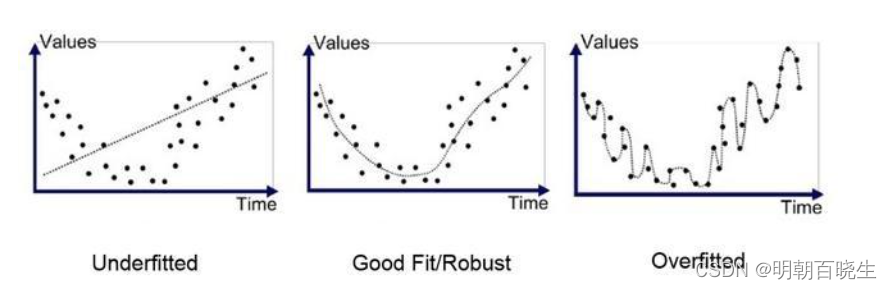
ERM 最小化原则往往会导致在训练集上面错误率很低，但是在测试集上面错误率很高，

这种就是过拟合（overfitting）

结构风险最小化（Structural Risk Minimization, SRM）

准则是为了防止过拟合而提出来的策略。过拟合问题往往是由于训练数据少和噪声以及模型能力强等原因造成的。为了解决过拟合问题，一般在经验风险最小化的基础上再引入参数的正则化（regularization），来限制模型能力，使其不要过度地最小化经验风险。

结构风险最小化等价于正则化。结构风险=经验风险+正则化项。在假设空间、损失函数以及训练集确定的情况下，结构风险的定义如下

$\theta^{*}=argmin_{\theta}R_{D}^{struct}(\theta)$

$=argmin_{\theta}R_{D}^{emp}(\theta)+\frac{1}{2}||\theta||^2$

$=argmin_{\theta}\frac{1}{N}\sum_{1}^{N}L(y^n,f(x^n;\theta))+\frac{1}{2}\lambda ||\theta||^2$

和过拟合相反的概念是欠拟合（Underfitting）,在训练集上的错误率很高，一般是模型能力不足导致的。

无优化算法

在确定了训练集D,假设空间F以及学习准则后，如何找到最优的模型 $f(x,\theta^*)$ 就

成立一个最优问题。

5.1 参数与超参数

在机器学习中，优化分为参数优化和超参数优化。模型 $f(x;\theta)$ 中

$\theta$ 称为模型的参数。

还有一类参数用来定义模型结构或优化策略的，这类参数叫做

超参数：步长，聚类类别个数，神经网络层数，支持向量机的核函数

5.2 梯度下降法（Batch Gradient Descent）

$\theta_{t+1}=\theta_t-\alpha \frac{\partial R_D}{\partial \theta}$

$=\theta_t -\alpha \frac{1}{N}\sum_{n=1}^{N}\frac{\partial L}{\partial \theta}$

$\alpha$ : 为搜索步长。

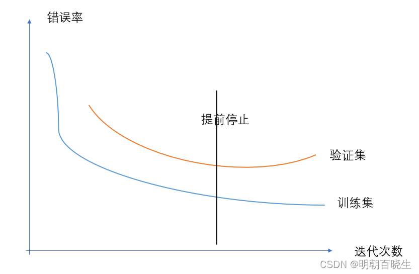
5.3 提前停止

在梯度下降训练过程中，由于过拟合的原因，在训练集上收敛的参数

并不一定在测试集上最优。因此除了训练集和测试集之外，有时会使用一个验证集

（Validation set）

每次迭代时，把得到的模型 $f(x;\theta)$ 在验证集上进行测试，并计算错误率。

如果在验证集上的错误率不再下降，就停止迭代。

如果没有验证集可以在训练集上划分一个小比例的子集作为验证集

5.4 随机梯度下降法(SGD stochastic Gradient Descent)

输入：训练集 $D=\begin{Bmatrix} {x^n,y^n} \end{Bmatrix}_{n=1}^{N}$

验证集 V

学习率 $\alpha$

随机初始化参数 $\theta$

对训练集D中的样本随机排序

for n = 1.....N do

从训练集中选取样本 $\begin{pmatrix} x^n,y^n \end{pmatrix}$

$\theta_{t+1}= \theta_{t}-\alpha \frac{\partial L(\theta_t;x^n,y^n)}{\partial \theta}$

end

until 模型 $f(x;\theta)$ 在验证集V上的错误率不再下降；

输出 $\theta$

批量梯度下降法和随机梯度下降法区别在于:

每次迭代的优化目标是针对所有的样本平均损失函数还是对单个样本的

损失函数。由于随机梯度下降实现简单，收敛速度非常快，因此应用广泛。

随机梯度下降在批量梯度下降的梯度上引入了噪声，在非凸问题中，更容易

逃离局部最优点。

5.5 小批量梯度下降法（Mini-Batch Gradient Descent）

这是批量梯度下降和随机梯度下降的这种。

每次训练时候，随机选取一小部分的样本来训练并计算梯度，并更新

参数，这样即可以兼顾梯度下降的优点又可以提高训练效率。

第 t次迭代时，随机选取一个包含K个样本的子集 $\delta_t$ ,并

计算这个子集上每个样本的损失函数的梯度平均值，然后更新参数

$\theta_{t+1}=\theta_{t}-\alpha \frac{1}{K}\sum_{\begin{pmatrix} x,y \end{pmatrix} \in \delta_t } \frac{\partial L}{\partial \theta}$

实际应用中，小批量随机梯度下降计算开销小，收敛快，因此逐渐成为主要的机器学习方法。

六线性回归例子

这边主要基于Numpy 和 Torch 实现一个线性回顾的简单例子

$\hat{y}=Xw+b$

输入：

X:[m,n] 的矩阵，维度为n, m为样本个数

w: [n,1]的向量，维度为n

输出

$\hat{y}$ : [m,1] 的预测值

损失函数

$loss =\frac{1}{2m}(Xw+b-y)^T(Xw+b-y)$

梯度：

$z= Xw+b-y$

${w}'=\frac{X^Tw}{m}$

${b}'=\frac{sum(z)}{m}$

6.1 python 版本

# -*- coding: utf-8 -*-
"""
Created on Sat May 14 05:47:25 2022

@author: cxf
"""

import numpy as np
import matplotlib.pyplot as plt

'''
获取数据
    y = xw+b
args:
    m: 样本个数
    n: 样本维度
'''
def getData(m,n):
    
    x = np.random.rand(m,n)
    w = np.array([1.0,1.0]).T
    b = 0.5 #偏置
    
    y = np.dot(x,w)+b
    
    
    return x,y.reshape(m,1)

'''
梯度计算
'''
def getGrad(pred_y, y, x,m):
    z = pred_y-y
    
    grad_w = np.dot(x.T, z)
    grad_b = np.sum(z)
    
    loss = np.sum(np.power(z,2))
    #print("\n ---w  ",grad_w)
    #print("\n ----z ",z)
    return grad_w/m, grad_b/m,loss

'''
m:样本个数
n: 样本维度
'''
def train(m,n):
    
    lr = 0.1 #学习率
    epoch = 50000 #最大迭代次数
    res =[] #存放损失函数的
    
    x,y = getData(m, n)
    w = np.random.rand(n,1) #w 初始化
    b = np.random.rand()
    #print("\n ---------------------\n")
    #print("\n w: \n ",w)
    #print("\n b: \n ",b)
    
    for step in range(epoch):
        
        pred_y = np.dot(x,w)+b
        grad_w, grad_b, loss = getGrad(pred_y, y,x,m)
        res.append(loss)
       
        w -= lr*grad_w
        b -= lr*grad_b
    print("\n w ",w,"\t b ",b)
    plt.plot(np.arange(0,len(res)),res)
    plt.show()
    
    
if __name__ == "__main__":   

    train(500,2)

6.2 torch 版本

# -*- coding: utf-8 -*-
"""
Created on Sun May 15 12:05:54 2022

@author: cxf
"""
import torch as t
import numpy as np
import matplotlib.pylab as plt
import os
#os.environ["KMP_DUPLICATE_LIB_OK"]="TRUE"



class linear():
    
    def __init__(self, m = 1000, n= 2, batch =100, epoch =300, lr = 0.1):
        self.m = m #样本个数
        self.n = n #样本维度
        self.batch = batch #批量样本个数
        self.epoch = epoch #迭代次数
        self.lr = lr #学习率
        self.w_true = t.Tensor([1.0,1.0]).view(n,1) #模型真实的权重系数
        self.b_true = t.Tensor([1.0]) #模型的偏置系数
        self.momentum = 0.5 #动量因子
        
    
    '''
    生成训练的数据集
    args:
        batch 生成训练的数据集
        
    return
       x: 训练的数据
       y: 标签值
    '''
    def load_data(self):
        
        x= t.randn(self.m,self.n)
        y = t.matmul(x,self.w_true)+self.b_true
        
        print("\n x_shape : ",x.shape, "\n y shape: ",y.shape)
        
        return x, y
    
    '''
    计算梯度
    args:
         pred_y: 预测值
         y:标签值
         x: 训练的数据
         
    '''
    def get_grad(self, pred_y,y,x,m):
        
        z= pred_y-y
        
        grad_w = t.matmul(x.T, z)/m
        grad_b = t.mean(z)
        
        loss = t.pow(z,2)*0.5 #损失值
        loss = t.sum(loss) #loss 求和
        
        
        
        return grad_w, grad_b,loss
    
    '''
    使用批量梯度下降
    args
       train_x: 总体训练样本
       train_y: 总体的标签
    return
       x: 数据
       y: 标签
    '''
    def get_data(self, train_x, train_y, batch):
        
        
    
          indices = t.randint(0,self.m,(batch,))
          x = t.index_select(train_x, dim=0, index= indices)
          y = t.index_select(train_y, dim=0, index= indices)
          print("\n indices ",indices, indices.shape)
        
          
          #print("\n x ",x.shape, "\t y ",y.shape, "\n train ",train_x.shape, train_y.shape)
          return x, y
        
    
    
    '''
    训练数据
    '''
    def train(self):
        t.manual_seed(5000) #随机数种子
        
        train_x,train_y = self.load_data()
        
        w= t.rand_like(self.w_true)
        b = t.rand_like(self.b_true)
        loss_record =[]
        
        #print("\n w:", w.shape)
        #print("\n b: ",b)
        
        
        for step in range(self.epoch):
            
            x,y = self.get_data(train_x, train_y, self.batch)
            
            #pred_y = t.matmul(train_x, w)+b
            pred_y = t.matmul(x, w)+b
            #print("\n pred_y sp",pred_y.shape)
            #a,b = self.get_data(train_x, train_y, self.batch)
            
            grad_w, grad_b,loss = self.get_grad(pred_y,y ,x,self.batch)
            print("\n loss ",loss)
            loss_record.append(loss)
            
            w -= self.lr*grad_w
            b -= self.lr*grad_b
        print("\n w ",w)
        print("\n b ",b)
        
        a = np.arange(0,self.epoch)
        
        plt.plot(a, loss_record)
        plt.show()
            
        


if __name__ =="__main__":
    
    ln = linear()
    
    ln.train()

明朝百晓生

关注

0
点赞
踩
0

收藏

觉得还不错? 一键收藏
0
评论
神经网络与深度学习-1- 机器学习概述-PyTorch

前言：《神经网络与深度学习》邱锡鹏https://www.bilibili.com/video/BV1Vx411j7kT?spm_id_from=333.337.search-card.all.clickhttps://www.bilibili.com/video/BV1Sr4y1N71H?spm_id_from=333.337.search-card.all.clickhttps://www.bilibili.com/video/BV1244y1G7B8?spm_id_from=...
复制链接

扫一扫