


chainer优势——边定义边运行
当下已有的深度学习框架使用的是“定义后运行”机制。即意味着,首先定义并且固化一个网络,再周而复始地馈入小批量数据进行训练。由于网络是在任何前向、反向计算前静态定义的,所有的逻辑作为数据必须事先嵌入网络中。 意味着,在诸如Caffe这样的框架中通过声明的方法定义网络结构。(注:可以使用torch.nn, 基于 Theano框架, 以及 TensorFlow 的命令语句定义一个静态网络)
Chainer 对应地采用了一种叫做 “边定义边运行” 的机制, 即, 网络可以在实际进行前向计算的时候同时被定义。 更加准确的说, Chainer 存储的是计算的历史结果而不是计算逻辑。这个策略使我们能够充分利用Python中编程逻辑的力量。例如,Chainer不需要任何魔法就可以将条件和循环引入到网络定义中。 边定义边运行是Chainer的核心概念。 我们将在本教程中展示如何动态定义网络。
这个策略也使编写多GPU并行化变得容易,因为逻辑更接近于网络操作。我们将在本教程后面的章节中回顾这些设施。
Chainer 将网络表示为计算图上的执行路径。计算图是一系列函数应用,因此它可以用多个Function对象来描述。当这个Function是一个神经网络层时,功能的参数将通过训练来更新。因此,该函数需要在内部保留可训练的参数,因此Chainer具有Link类,它可以在类的对象上保存可训练参数。在Link对象中执行的函数的参数被表示为Variable对象。 简言之,Link和Function之间的区别在于它是否包含可训练参数。 神经网络模型通常被描述为一系列Link和Function。
您可以通过动态“链接”各种Link和Function来构建计算图来定义Chain。在框架中,通过运行链接图来定义网络,因此名称是Chainer。
前向/反向计算,连接、模型、优化器、训练器、序列化器、多层感知器
chainer搭建网络架构的方式
示例1:编码器
class Encoder_text_tower(chainer.Chain):
    """
    An implementation of the "Tower" model of the VAE encoder from the paper
    'Neural scene representation and rendering, by S. M. Ali Eslami and others at DeepMind.
    The exact numbers of the layers and were changed.

    It is basically a cVAE with multi-dimensional conditions.

    v - human level properties HLP, human classification ???? find a good name

    This system takes as input an image and two one-hot vectors corresponding to factorized
    features of the main object encoded in the image. For instance, if the image contains a
    red sphere, the inputs will <image>,"red","round".

    Intent: The hypothesis is that by providing HLPs during training and also during testing,
    we get a better encoding _of the particular object_.

    Validation: We can check the reconstruction error metric, but we can also check this
    with visual inspection of the reconstructed version for different HLP inputs
    """
    '''
    2023.2.13 11.30
    '''
    # 变分自编码器
    def __init__(self, density=1, size=64, latent_size=100, channel=3, att_size=32, hidden_dim=100, num_objects=10, num_descriptions=10):
        """
        density - a scaling factor for the number of channels in the convolutional layers. It is multiplied by at least
        16,32,64 and 128 as we go deeper.
        Use: using density=8 when training the VAE separately. using density=4 when training end to end
        Intent: increase the number of features in the convolutional layers.
        """
        assert (size % 16 == 0) # 其作用是如果它的条件返回错误,则终止程序执行.判断size是不是16的倍数
        self.att_size = att_size
        self.density = density
        self.second_size = size // 4  # //表示整除,返回商的整数部分(向下取整)
        initial_size = size // 16
        # 预先定义一些可能用到的神经网络层,整个网络架构在__call__这个函数体现
        super(Encoder_text_tower, self).__init__(
            # 10+10——16*16*7
            toConv=L.Linear(num_objects + num_descriptions, self.second_size * self.second_size * 7, initialW=Normal(0.02)),

            dc1=L.Convolution2D(channel, int(16 * density), 3, stride=2, pad=1,
                                initialW=Normal(0.02)),
            dc2=L.Convolution2D(int(16 * density), int(32 * density), 3, stride=2, pad=1,
                                initialW=Normal(0.02)),
            dc1_=L.Convolution2D(int(16 * density), int(16 * density), 3, stride=1, pad=1,
                                initialW=Normal(0.02)),
            dc2_=L.Convolution2D(int(32 * density), int(32 * density), 3, stride=1, pad=1,
                                initialW=Normal(0.02)),
            # 批标准化:BatchNorm就是在深度神经网络训练过程中使得每一层神经网络的输入保持相同分布的。
            # BN的基本思想其实相当直观:
            # 因为深层神经网络在做非线性变换之前的激活输入值(z = wx +b,x是输入,z是非线性函数输入值)
            # 随着网络深度加深或者在训练过程中,其分布逐渐发生偏移或者移动,
            # 之所以训练收敛变慢,一般是整体分布逐渐往非线性函数的取值区间的上下两端靠近(对于sigmoid函数来说,意味着激活输入值z是大的负值或正值),
            # 所以这导致反向传播时底层神经网络的梯度消失,这是训练神经网络收敛越来越慢的本质原因,
            # 而BN就是通过一定的规范化手段,把每层神经网络任意神经元这个输入值的分布强行拉回到均值为0方差为1的标准正态分布,
            # 其实就是把越来越偏的分布强制拉回比较标准的分布,这样使得激活输入值落在非线性函数对输入比较敏感的区域,
            # 这样输入的小变化就会导致损失函数较大的变化,意思是这样让梯度变大,避免梯度消失问题产生,
            # 而且梯度变大意味着学习收敛速度快,能大大加快训练速度。其实一句话就是:对于每个隐层神经元,
            # 把逐渐向非线性函数映射后取值区间极限饱和区靠拢的输入分布 强制拉回到均值为0方差为1的比较标准的正态分布,
            # 使得非线性变换的输入值落入对输入比较敏感的区域,以此避免梯度消失问题。因为梯度一直能保存比较大的状态,所以很明显对神经网络的参数调整效率比较高,
            # 就是变动大,就是说像损失函数最优值迈动的步子大,也就是收敛的快。
            norm2=L.BatchNormalization(int(32 * density)),
            norm2_=L.BatchNormalization(int(32 * density)),
            dc2_p=L.Convolution2D(int(32 * density), int(32 * density), 3, stride=1, pad=1,
                                initialW=Normal(0.02)),
            norm2_p=L.BatchNormalization(int(32 * density)),
            dc3=L.Convolution2D(int(32 * density), int(64 * density), 3, stride=2, pad=1,
                                initialW=Normal(0.02)),
            norm3=L.BatchNormalization(int(64 * density)),
            dc3_=L.Convolution2D(int(64 * density), int(64 * density), 3, stride=1, pad=1,
                                initialW=Normal(0.02)),
            norm3_=L.BatchNormalization(int(64 * density)),
            dc3_p=L.Convolution2D(int(64 * density), int(64 * density), 3, stride=1, pad=1,
                                initialW=Normal(0.02)),
            norm3_p=L.BatchNormalization(int(64 * density)),
            dc4=L.Convolution2D(int(64 * density), int(128 * density), 3, stride=1, pad=1,
                                initialW=Normal(0.02)),
            norm4=L.BatchNormalization(int(128 * density)),
            norm_toConv=L.BatchNormalization(7),

            fc_video0 = L.Convolution2D(int(128 * density), int(128 * density), 1, stride=1, pad=0, initialW=Normal(0.02), nobias=True),
            norm0 = L.BatchNormalization(int(128 * density), use_gamma = False),
            fc_video1 = L.Convolution2D(int(128 * density), int(8 * density), 1, stride=1, pad=0, initialW=Normal(0.02), nobias=True),
            norm1 = L.BatchNormalization(int(8 * density), use_gamma = False),
            fc_video2 = L.Convolution2D(int(8 * density), int(8 * density), 1, stride=1, pad=0, initialW=Normal(0.02)),

            # Text Input Layers
            fc_text0 = L.Linear(num_objects + num_descriptions, int(8 * density), initialW=Normal(0.02), nobias=True),
            norm_text0 = L.BatchNormalization(int(8 * density)),
            fc_text1 = L.Linear(int(8 * density), int(8 * density), initialW=Normal(0.02)),

            #Attention Extraction
            norm_mix = L.BatchNormalization(int(8 * density), use_gamma = False),
            fc_mix0 = L.Convolution2D(int(8 * density), 1, 1, stride=1, pad=0, initialW=Normal(0.02)),

            #Classifier
            fc_cls0 = L.Linear(int(128 * density), int(32 * density), initialW=Normal(0.02), nobias=True),
            norm_cls0 = L.BatchNormalization(int(32 * density)),
            fc5 = L.Linear(int(32 * density), num_objects + 1, initialW=Normal(0.02)),
            fc6 = L.Linear(int(32 * density), num_descriptions + 1, initialW=Normal(0.02)),
        )

    def __call__(self, x, objects_one_hot, descs_one_hot, train=True):
        with chainer.using_config('train', train), chainer.using_config('enable_backprop', train):
            # 其实就是描述整个前向传播的过程
            xp = cuda.get_array_module(x.data)
            h1 = F.leaky_relu(self.dc1(x))
            h1_ = F.leaky_relu(self.dc1_(h1))
            h2 = F.leaky_relu(self.norm2(self.dc2(h1_)))
            h2_ = F.leaky_relu(self.norm2_(self.dc2_(h2)))
            h2_p = F.leaky_relu(self.norm2_p(self.dc2_p(h2_)))
            h2_pp = h2_ + h2_p
            # h2_pp = F.concat((h2_pp, h0), axis=1)
            h3 = F.leaky_relu(self.norm3(self.dc3(h2_pp)))
            h3_ = F.leaky_relu(self.norm3_(self.dc3_(h3)))
            h3_p = F.leaky_relu(self.norm3_p(self.dc3_p(h3)))
            h3_ = h3_ + h3_p
            h4 = F.leaky_relu(self.norm4(self.dc4(h3_)))

            f0 = F.leaky_relu(self.norm0(self.fc_video0(h4)))
            f1 = F.leaky_relu(self.norm1(self.fc_video1(f0)))
            f3 = self.fc_video2(f1)

            s0 = F.leaky_relu(self.norm_text0(self.fc_text0(F.concat((objects_one_hot, descs_one_hot), axis=-1))))
            s1 = self.fc_text1(s0)
            s2 = F.expand_dims(s1, axis=2)
            s2 = F.repeat(s2, self.att_size * self.att_size, axis=2)
            s2 = F.reshape(s2, (-1, int(8 * self.density), self.att_size, self.att_size))

            m3 = f3 + s2
            m3 = F.tanh(self.norm_mix(m3))
            m4 = F.reshape(self.fc_mix0(m3), (-1, self.att_size * self.att_size))
            m4 = F.sigmoid(m4)
            m4 = 100 * F.normalize(F.relu(m4 - 0.5), axis=1)
            m4 = F.clip(m4, 0.0, 1.0)

            h4 = F.reshape(h4, (-1, int(self.density * 128), self.att_size * self.att_size))

            if train:
                features = F.einsum('ijk,ik -> ij', h4, m4)
            else:
                features = F.einsum('ijk,ik -> ij', h4, m4)
            #Classifier
            t0 = self.norm_cls0(F.leaky_relu(self.fc_cls0(features)))
            s2 = self.fc5(t0)
            c2 = self.fc6(t0)

            return m4, s2, c2
示例2:简单神经网络
import chainer
import numpy as np

class ChainerCnn(chainer.Chain):
    def __init__(self,gakushuuritsu):
        super(ChainerCnn,self).__init__()
        with self.init_scope():
            self.c1 = chainer.links.Convolution2D(1,16,5,1,2)
            self.c2 = chainer.links.Convolution2D(16,32,5,1,2)
            self.l1 = chainer.links.Linear(1568,16)
            self.l2 = chainer.links.Linear(16,10)
        self.opt = chainer.optimizers.Adam(gakushuuritsu)
        self.opt.setup(self)

    def __call__(self,x):
        x = self.c1(x)
        x = chainer.functions.relu(x)
        x = chainer.functions.max_pooling_2d(x,2)
        x = self.c2(x)
        x = chainer.functions.relu(x)
        x = chainer.functions.max_pooling_2d(x,2)
        x = self.l1(x)
        x = chainer.functions.relu(x)
        x = self.l2(x)
        return x

    def gakushuu(self,X_kunren,y_kunren,X_kenshou,y_kenshou,kurikaeshi,n_batch):
        n_kunren = len(y_kunren)
        X_kunren = X_kunren.reshape(-1,1,28,28).astype(np.float32)
        y_kunren = y_kunren.astype(np.int32)
        X_kenshou = X_kenshou.reshape(-1,1,28,28).astype(np.float32)
        y_kenshou = y_kenshou.astype(np.int32)

        print(u'==chainer学習開始==')
        t_kaishi = time.time()
        for j in range(kurikaeshi):
            batch = np.random.permutation(n_kunren)
            for i in range(0,n_kunren,n_batch):
                Xn = X_kunren[batch[i:i+n_batch]]
                yn = y_kunren[batch[i:i+n_batch]]
                loss = chainer.functions.softmax_cross_entropy(self(Xn),yn)
                self.cleargrads()
                loss.backward()
                self.opt.update()
            seikaku = (chainer.functions.argmax(self(X_kenshou),1).data==y_kenshou).mean()
            print(u'%d回目 正確度%.4f もう%.3f分かかった'%(j+1,seikaku,(time.time()-t_kaishi)/60))
pytorch搭建网络的方式
示例1
import torch
import time

relu = torch.nn.ReLU()
entropy = torch.nn.CrossEntropyLoss()
pool = torch.nn.MaxPool2d(2)

class PytorchCnn(torch.nn.Module):
    def __init__(self,gakushuuritsu):
        super(PytorchCnn,self).__init__()
        self.c1 = torch.nn.Conv2d(1,16,5,1,2)
        self.c2 = torch.nn.Conv2d(16,32,5,1,2)
        self.l1 = torch.nn.Linear(1568,16)
        self.l2 = torch.nn.Linear(16,10)
        self.opt = torch.optim.Adam(self.parameters(),lr=gakushuuritsu)

    def forward(self,x):
        x = self.c1(x)
        x = relu(x)
        x = pool(x)
        x = self.c2(x)
        x = relu(x)
        x = pool(x)
        x = x.view(x.size()[0],-1)
        x = self.l1(x)
        x = relu(x)
        x = self.l2(x)
        return x

    def gakushuu(self,X_kunren,y_kunren,X_kenshou,y_kenshou,kurikaeshi,n_batch):
        n_kunren = len(y_kunren)
        X_kunren = torch.FloatTensor(X_kunren.reshape(-1,1,28,28))
        y_kunren = torch.LongTensor(y_kunren)
        X_kenshou = torch.FloatTensor(X_kenshou.reshape(-1,1,28,28))
        y_kenshou = torch.LongTensor(y_kenshou)

        print(u'==pytorch学習開始==')
        t_kaishi = time.time()
        for j in range(kurikaeshi):
            batch = torch.randperm(n_kunren)
            for i in range(0,n_kunren,n_batch):
                Xn = X_kunren[batch[i:i+n_batch]]
                yn = y_kunren[batch[i:i+n_batch]]
                loss = entropy(self(Xn),yn)
                self.opt.zero_grad()
                loss.backward()
                self.opt.step()
            seikaku = (self(X_kenshou).argmax(1)==y_kenshou).type(torch.FloatTensor).mean().item()
            print(u'%d回目 正確度%.4f もう%.3f分かかった'%(j+1,seikaku,(time.time()-t_kaishi)/60))
示例2
class MyModel(nn.Module):
    def __init__(self):
        super(MyModel, self).__init__()
        self.linear1 = nn.Linear(10, 64) # 线性层
        self.activation = nn.ReLU()
        self.linear2 = nn.Linear(64, 8)
        self.linear3 = nn.Linear(8, 4)

    def forward(self, x):

        output = self.linear1(x)  # [batch_size, 64]
        output = self.activation(output)  # [batch_size, 64]
        output = self.linear2(output)  # [batch_size, 8]
        output = self.linear3(output)  # [batch_size, 4]
        return output
chainer.links.Convolution2D()
classchainer.links.Convolution2D(self, in_channels, out_channels, ksize=None, stride=1, pad=0, nobias=False, initialW=None, initial_bias=None, *, dilate=1, groups=1)
in_channels (int or None) – Number of channels of input arrays. If None, parameter initialization will be deferred until the first forward data pass at which time the size will be determined.
out_channels (int) – Number of channels of output arrays.
ksize (int or pair of ints) – Size of filters (a.k.a. kernels). ksize=k and ksize=(k, k) are equivalent.
stride (int or pair of ints) – Stride of filter applications. stride=s and stride=(s, s) are equivalent.
pad (int or pair of ints) – Spatial padding width for input arrays. pad=p and pad=(p, p) are equivalent.
nobias (bool) – If True, then this link does not use the bias term.
initialW (initializer) – Initializer to initialize the weight. When it is numpy.ndarray, its ndim should be 4.
initial_bias (initializer) – Initializer to initialize the bias. If None, the bias will be initialized to zero. When it is numpy.ndarray, its ndim should be 1.
dilate (int or pair of ints) – Dilation factor of filter applications. dilate=d and dilate=(d, d) are equivalent.
groups (int) – Number of groups of channels. If the number is greater than 1, input tensor W is divided into some blocks by this value channel-wise. For each tensor blocks, convolution operation will be executed independently. Input channel size in_channels and output channel size out_channels must be exactly divisible by this value.
class VGG(chainer.Chain):
    def __init__(self):
        super(VGG, self).__init__(
            conv1_1=L.Convolution2D(3, 64, 3, stride=1, pad=1),
            conv1_2=L.Convolution2D(64, 64, 3, stride=1, pad=1),

            conv2_1=L.Convolution2D(64, 128, 3, stride=1, pad=1),
            conv2_2=L.Convolution2D(128, 128, 3, stride=1, pad=1),

            conv3_1=L.Convolution2D(128, 256, 3, stride=1, pad=1),
            conv3_2=L.Convolution2D(256, 256, 3, stride=1, pad=1),
            conv3_3=L.Convolution2D(256, 256, 3, stride=1, pad=1),

            conv4_1=L.Convolution2D(256, 512, 3, stride=1, pad=1),
            conv4_2=L.Convolution2D(512, 512, 3, stride=1, pad=1),
            conv4_3=L.Convolution2D(512, 512, 3, stride=1, pad=1),

            conv5_1=L.Convolution2D(512, 512, 3, stride=1, pad=1),
            conv5_2=L.Convolution2D(512, 512, 3, stride=1, pad=1),
            conv5_3=L.Convolution2D(512, 512, 3, stride=1, pad=1)
        )
        self.train = False
        self.mean = np.asarray(120, dtype=np.float32)

    def preprocess(self, image):
        return np.rollaxis(image - self.mean, 2)

    def __call__(self, x):
        y1 = F.relu(self.conv1_2(F.relu(self.conv1_1(x))))
        h = F.max_pooling_2d(y1, 2, stride=2)
        y2 = F.relu(self.conv2_2(F.relu(self.conv2_1(h))))
        h = F.max_pooling_2d(y2, 2, stride=2)
        y3 = F.relu(self.conv3_3(F.relu(self.conv3_2(F.relu(self.conv3_1(h))))))
        h = F.max_pooling_2d(y3, 2, stride=2)
        y4 = F.relu(self.conv4_3(F.relu(self.conv4_2(F.relu(self.conv4_1(h))))))
        return [y1, y2, y3, y4]
conv=L.Convolution2D(in_channels, out_channels, ksize, stride, pad)
# in_channels  输入通道数
# out_channels 输出通道数
# ksize  卷积核大小
# stride  步长
# pad  填充
在机器学习领域中,通道数一般表示非图片尺寸维度,比如彩色图片通道数为3,黑白图片或灰度图通道数为1,卷积后图片通道数由卷积核数量(卷积次数)决定。
chainer.links.BatchNormalization()
classchainer.links.BatchNormalization(size=None, decay=0.9, eps=2e-05, dtype=None, use_gamma=True, use_beta=True, initial_gamma=None, initial_beta=None, axis=None, initial_avg_mean=None, initial_avg_var=None)
size (int, tuple of ints, or None) – Size (or shape) of channel dimensions. If None, the size will be determined from dimension(s) of the input batch during the first forward pass.
decay (float) – Decay rate of moving average. It is used on training.
eps (float) – Epsilon value for numerical stability.
dtype (numpy.dtype) – Type to use in computing.
use_gamma (bool) – If True, use scaling parameter. Otherwise, use unit(1) which makes no effect.
use_beta (bool) – If True, use shifting parameter. Otherwise, use unit(0) which makes no effect.
axis (int or tuple of int) – Axis over which normalization is performed. When axis is None, it is determined from input dimensions. For example, if x.ndim is 4, axis becomes (0, 2, 3) and normalization is performed over 0th, 2nd and 3rd axis of input. If it is 2, axis becomes (0) and normalization is performed over 0th axis of input. When a tuple of int is given to this option, numbers in the tuple must be being sorted in ascending order. For example, (0, 2) is OK, but (2, 0) is not.
initial_gamma – Initializer of the scaling parameter. The default value is 1.
initial_beta – Initializer of the shifting parameter. The default value is 0.
initial_avg_mean – Initializer of the moving average of population mean. The default value is 0.
initial_avg_var – Initializer of the moving average of population variance. The default value is 1.
norm=L.BatchNormalization(32)
argparse.ArgumentParser()用法解析
1、介绍
argparse是python用于解析命令行参数和选项的标准模块,用于代替已经过时的optparse模块。argparse模块的作用是用于解析命令行参数。
我们很多时候,需要用到解析命令行参数的程序,目的是在终端窗口(ubuntu是终端窗口,windows是命令行窗口)输入训练的参数和选项。
2、使用步骤
我们常常可以把argparse的使用简化成下面四个步骤
import argparse

parser = argparse.ArgumentParser()

parser.add_argument()

parser.parse_args()
上面四个步骤解释如下:首先导入该模块;然后创建一个解析对象;然后向该对象中添加你要关注的命令行参数和选项,每一个add_argument方法对应一个你要关注的参数或选项;最后调用parse_args()方法进行解析;解析成功之后即可使用。
3、例子讲解
下面我们通过一个例子来进行讲解说明
我们可以看到上面的第二个步骤,parser = argparse.ArgumentParser()
它的作用就是:当调用parser.print_help()或者运行程序时由于参数不正确(此时python解释器其实也是调用了pring_help()方法)时,会打印这些描述信息,一般只需要传递description参数。
下面会有例子输出,首先给出代码:
#-*- coding: UTF-8 -*-
import argparse #步骤一
def parse_args():
"""
:return:进行参数的解析
"""
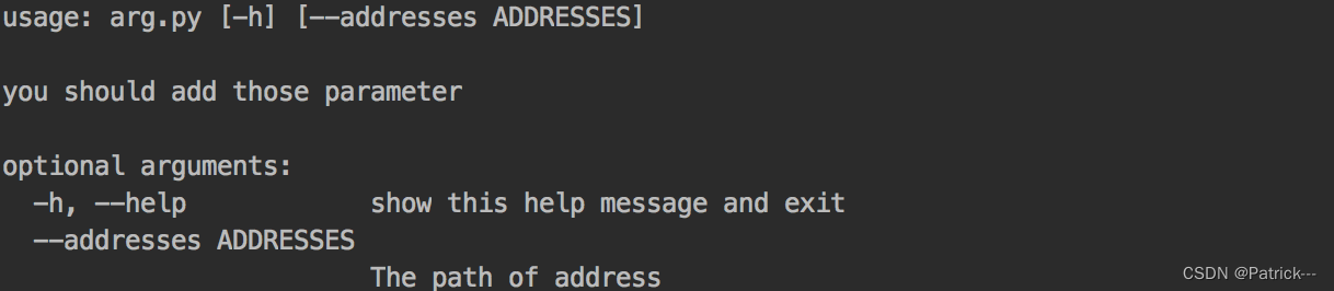
parser = argparse.ArgumentParser(description="you should add those parameter") # 这些参数都有默认值,当调用parser.print_help()或者运行程序时由于参数不正确(此时python解释器其实也是调用了pring_help()方法)时, # 会打印这些描述信息,一般只需要传递description参数,如上。
parser.add_argument('--addresses',default="sipingroad", help = "The path of address")
parser.add_argument('--gpu', default=0)# 步骤二,后面的help是我的描述
args = parser.parse_args() # 步骤三
return args
if __name__ == '__main__':
args = parse_args()
print(args.addresses) #直接这么获取即可。
chainer.using_config控制训练 or 预测?
使用方法1:直接赋值
chainer.config.train = False
here, code runs in the test mode, and dropout won't drop any unit.
model(x)
chainer.config.train = True
使用方法2:with using_config(key, value)符号
with chainer.using_config('train', False):
    # train config is set to False, thus code runs in the test mode.
    model(x)

# Here, train config is recovered to original value.
如果您使用trainer moudule,Evaluator将在验证/评估期间自动处理这些配置(请参阅document或source code)。这意味着train config设置为False,dropout在计算验证丢失时作为评估模式运行。


 307
307

 被折叠的 条评论
为什么被折叠?
被折叠的 条评论
为什么被折叠?
 到【灌水乐园】发言


