跟着Seurat官网学空间转录组（Slide-seq数据集为例）

Slide-seq版本

数据集

在这里，我们将分析使用小鼠海马体的Slide-seq v2生成的数据集。本教程将遵循与 10x Visium 数据的空间小插图大部分相同的结构，但专为提供特定于 Slide-seq 数据的演示而定制。

您可以使用我们的SeuratData 包来轻松访问数据，如下所示。安装数据集后，您可以键入?ssHippo以查看用于创建 Seurat 对象的命令。

InstallData("ssHippo")
slide.seq <- LoadData("ssHippo")

数据预处理

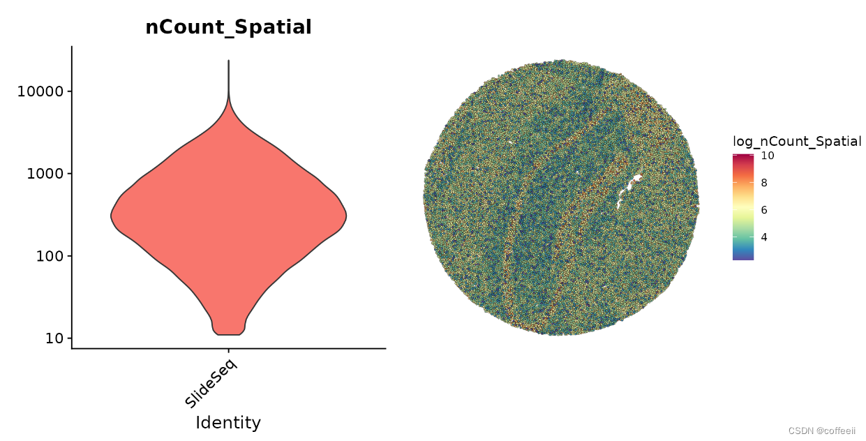
基因表达数据对珠子的初始预处理步骤类似于其他空间 Seurat 分析和典型的 scRNA-seq 实验。在这里，我们注意到许多珠子的 UMI 计数特别低，但选择保留所有检测到的珠子用于下游分析。

plot1 <- VlnPlot(slide.seq, features = "nCount_Spatial", pt.size = 0, log = TRUE) + NoLegend()
slide.seq$log_nCount_Spatial <- log(slide.seq$nCount_Spatial)
plot2 <- SpatialFeaturePlot(slide.seq, features = "log_nCount_Spatial") + theme(legend.position = "right")
wrap_plots(plot1, plot2)

然后，我们使用sctransform对数据进行标准化，并执行标准的 scRNA-seq 降维和聚类工作流程。

slide.seq <- SCTransform(slide.seq, assay = "Spatial", ncells = 3000, verbose = FALSE)
slide.seq <- RunPCA(slide.seq)
slide.seq <- RunUMAP(slide.seq, dims = 1:30)
slide.seq <- FindNeighbors(slide.seq, dims = 1:30)
slide.seq <- FindClusters(slide.seq, resolution = 0.3, verbose = FALSE)

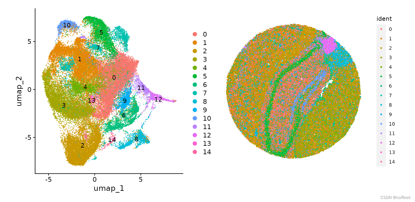
DimPlot()然后，我们可以在 UMAP 空间（带有）或珠子坐标空间中使用 可视化聚类的结果SpatialDimPlot()。

plot1 <- DimPlot(slide.seq, reduction = "umap", label = TRUE)
plot2 <- SpatialDimPlot(slide.seq, stroke = 0)
plot1 + plot2

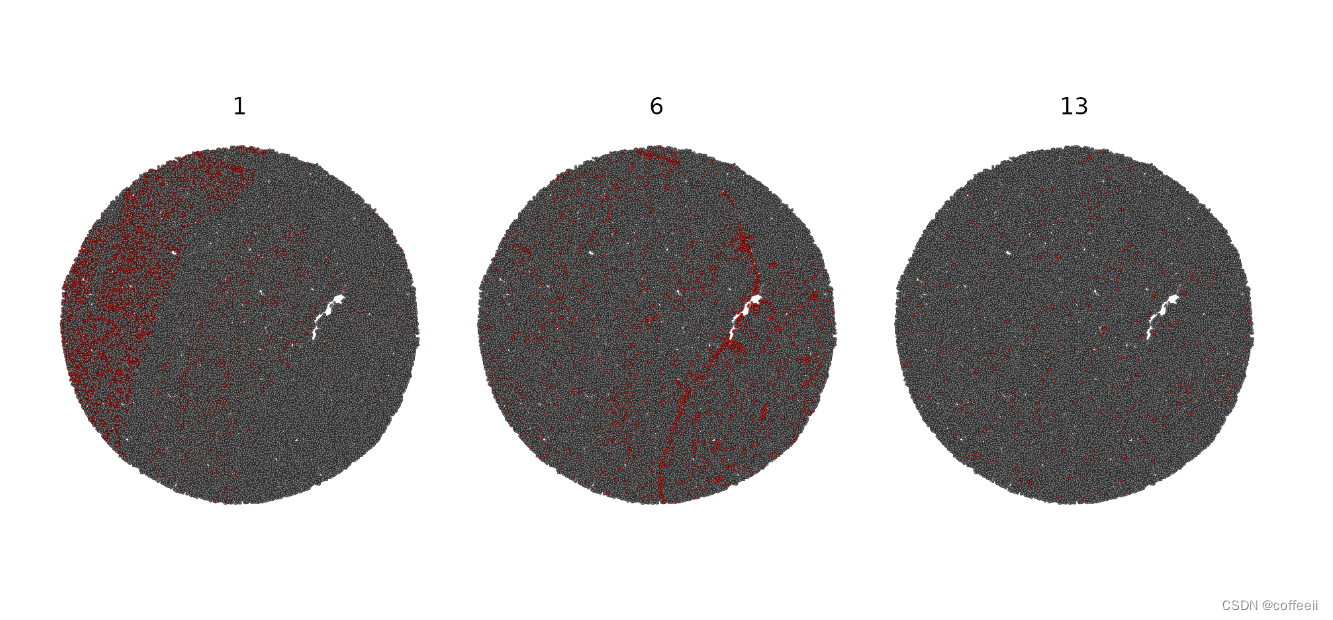
SpatialDimPlot(slide.seq, cells.highlight = CellsByIdentities(object = slide.seq, idents = c(1,
    6, 13)), facet.highlight = TRUE)

与 scRNA-seq 参考集成

为了促进 Slide-seq 数据集的细胞类型注释，我们正在利用Saunders*、Macosko* 等人生产的现有小鼠单细胞 RNA-seq 海马数据集。2018 年。数据可作为处理后的 Seurat 对象下载，原始计数矩阵可在DropViz 网站上获得。

ref <- readRDS("../data/mouse_hippocampus_reference.rds")
ref <- UpdateSeuratObject(ref)

论文的原始注释在 Seurat 对象的单元格元数据中提供。这些注释在几个“分辨率”中提供，从广泛的类别 ( ref$class)到细胞类型(ref$subcluster) 中的子集群。出于此小插图的目的，我们将对细胞类型注释 ( ) 进行修改ref$celltype，我们认为它取得了很好的平衡。

我们将首先运行 Seurat 标签转移方法来预测每个珠子的主要细胞类型。

anchors <- FindTransferAnchors(reference = ref, query = slide.seq, normalization.method = "SCT",
    npcs = 50)
predictions.assay <- TransferData(anchorset = anchors, refdata = ref$celltype, prediction.assay = TRUE,
    weight.reduction = slide.seq[["pca"]], dims = 1:50)
slide.seq[["predictions"]] <- predictions.assay

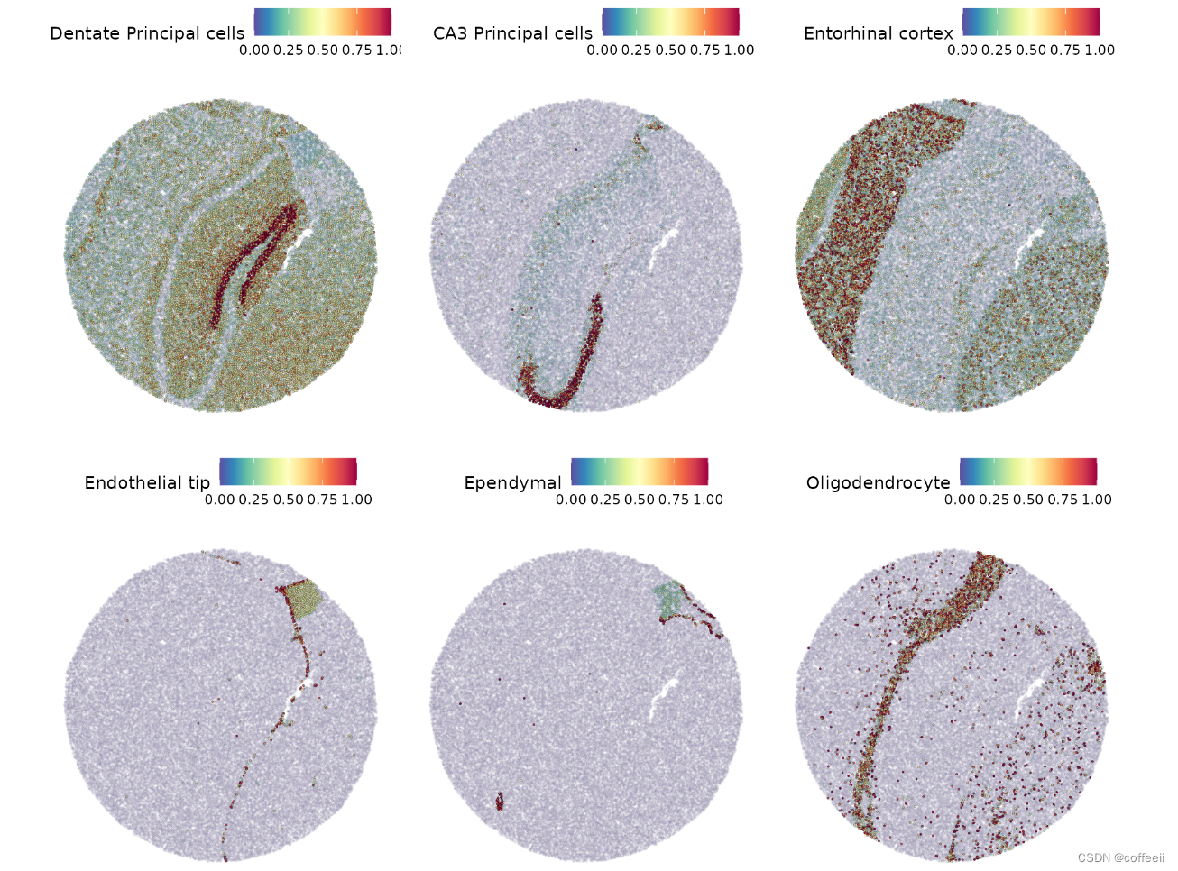
然后我们可以可视化一些主要预期类别的预测分数。

DefaultAssay(slide.seq) <- "predictions"
SpatialFeaturePlot(slide.seq, features = c("Dentate Principal cells", "CA3 Principal cells", "Entorhinal cortex",
    "Endothelial tip", "Ependymal", "Oligodendrocyte"), alpha = c(0.1, 1))

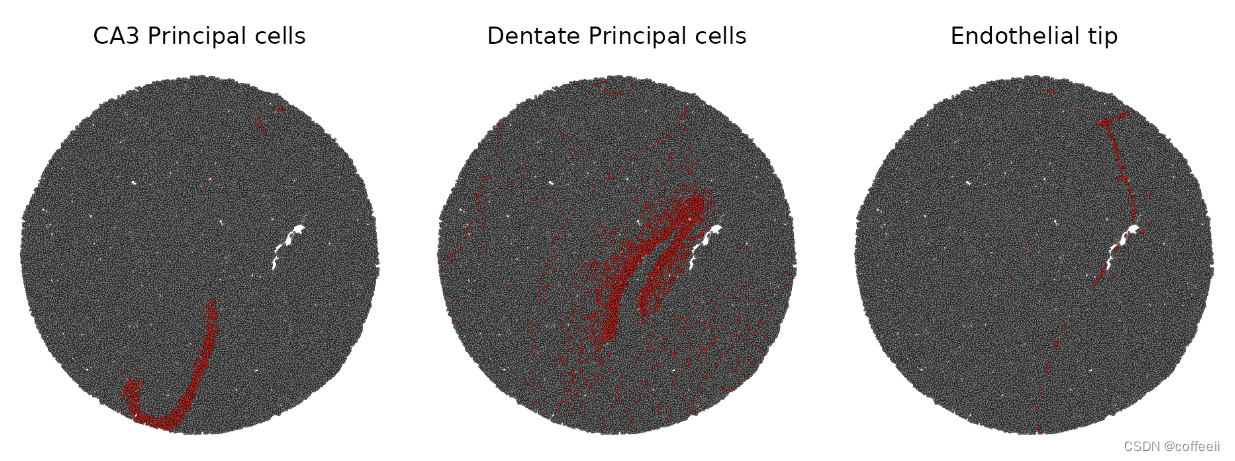
slide.seq$predicted.id <- GetTransferPredictions(slide.seq)
Idents(slide.seq) <- "predicted.id"
SpatialDimPlot(slide.seq, cells.highlight = CellsByIdentities(object = slide.seq, idents = c("CA3 Principal cells",
    "Dentate Principal cells", "Endothelial tip")), facet.highlight = TRUE)

空间可变特征的识别

正如 Visium v​​ignette 中提到的，我们可以通过两种一般方式识别空间可变特征：预先注释的解剖区域之间的差异表达测试或测量特征对空间位置的依赖性的统计数据。

FindSpatiallyVariableFeatures()在这里，我们通过设置提供 Moran’s I 的实现来演示后者method = ‘moransi’。Moran’s I 计算整体空间自相关并给出一个统计量（类似于相关系数）来衡量特征对空间位置的依赖性。这使我们能够根据特征的表达在空间上的变化程度对特征进行排名。为了便于快速估计此统计数据，我们实施了一个基本的分箱策略，该策略将在 Slide-seq 圆盘上绘制一个矩形网格，并对每个分箱内的特征和位置进行平均。x 和 y 方向的 bin 数量分别由x.cuts和y.cuts参数控制。此外，虽然不是必需的，但安装可选Rfast2包（install.packages(‘Rfast2’)), 将通过更有效的实施显着减少运行时间。

DefaultAssay(slide.seq) <- "SCT"
slide.seq <- FindSpatiallyVariableFeatures(slide.seq, assay = "SCT", slot = "scale.data", features = VariableFeatures(slide.seq)[1:1000],
    selection.method = "moransi", x.cuts = 100, y.cuts = 100)

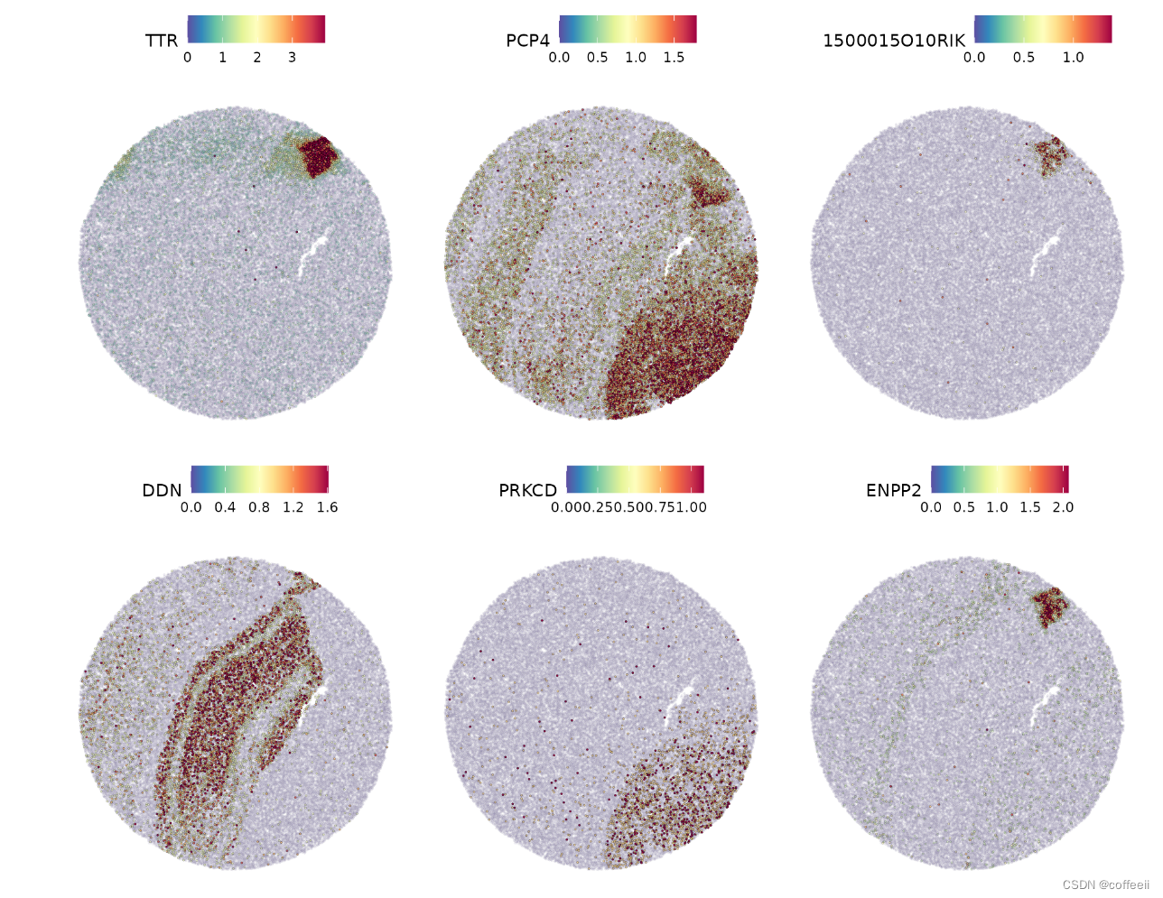
现在我们可视化 Moran’s I 识别的前 6 个特征的表达。

SpatialFeaturePlot(slide.seq, features = head(SpatiallyVariableFeatures(slide.seq, selection.method = "moransi"),
    6), ncol = 3, alpha = c(0.1, 1), max.cutoff = "q95")

SpatialFeaturePlot(slide.seq, features = head(SpatiallyVariableFeatures(slide.seq, selection.method = "moransi"),
    6), ncol = 3, alpha = c(0.1, 1), max.cutoff = "q95")

使用 RCTD 的空间反卷积

虽然FindTransferAnchors可用于整合来自空间转录组数据集的点级数据，但 Seurat v5 还包括对稳健细胞类型分解的支持，这是一种在提供 scRNA-seq 参考时从空间数据集中解卷积点级数据的计算方法。RCTD 已被证明可以准确地注释来自各种技术的空间数据，包括 SLIDE-seq、Visium 和 10x Xenium 原位空间平台。

要运行 RCTD，我们首先spacexr从实现 RCTD 的 GitHub 安装包。

devtools::install_github("dmcable/spacexr", build_vignettes = FALSE)

从 Seurat 查询和参考对象中提取计数、聚类和点信息以构建ReferenceRCTDSpatialRNA使用的对象进行注释。

library(spacexr)

# set up reference
ref <- readRDS("../data/mouse_hippocampus_reference.rds")
ref <- UpdateSeuratObject(ref)
Idents(ref) <- "celltype"

# extract information to pass to the RCTD Reference function
counts <- ref[["RNA"]]$counts
cluster <- as.factor(ref$celltype)
names(cluster) <- colnames(ref)
nUMI <- ref$nCount_RNA
names(nUMI) <- colnames(ref)
reference <- Reference(counts, cluster, nUMI)

# set up query with the RCTD function SpatialRNA
slide.seq <- SeuratData::LoadData("ssHippo")
counts <- slide.seq[["Spatial"]]$counts
coords <- GetTissueCoordinates(slide.seq)
colnames(coords) <- c("x", "y")
coords[is.na(colnames(coords))] <- NULL
query <- SpatialRNA(coords, counts, colSums(counts))

使用referenceandquery对象，我们注释数据集并将细胞类型标签添加到查询 Seurat 对象。RCTD 并行化很好，因此可以指定多个内核以获得更快的性能。

RCTD <- create.RCTD(query, reference, max_cores = 8)
RCTD <- run.RCTD(RCTD, doublet_mode = "doublet")
slide.seq <- AddMetaData(slide.seq, metadata = RCTD@results$results_df)

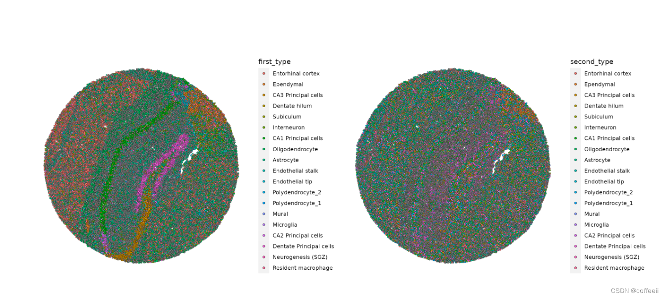
接下来，绘制 RCTD 注释。因为我们在 doublet 模式下运行 RCTD，算法会为每个条形码或点分配一个first_type和。second_type

p1 <- SpatialDimPlot(slide.seq, group.by = "first_type")
p2 <- SpatialDimPlot(slide.seq, group.by = "second_type")
p1 | p2

保存

write.csv(x = t(as.data.frame(all_times)), file = "../output/timings/spatial_vignette_times.csv")