


December is only 2 days away, so it's time for an Excel Advent Calendar! I've made two new versions this year, and they don't use macros, just basic Excel features. Even if you don't need an Advent calendar, take a look to see how they're set up . You might find a use for these techniques in other projects.
12月只有2天,所以现在该是一个Excel Advent Calendar了! 我今年已经制作了两个新版本,它们不使用宏,而仅使用基本的Excel功能。 即使您不需要Advent日历,也请看看它们的设置方式。 您可能会在其他项目中找到这些技术的用途。
花式日历 (Fancy Calendars)
When our kids were young, they got an Advent Calendar every December, with 24 numbered doors, and a small chocolate treat behind each door.
当我们的孩子还很小的时候,他们每年12月都有一个降临日历 ,上面有24个编号的门,每扇门后面都有一个小巧的巧克力点心。
In past years, I've shared Excel Advent calendars with Christmas pictures instead of chocolate. Those calendars had macros, to show each day's "treat".
在过去的几年中,我与圣诞节图片而不是巧克力共享Excel Advent日历。 这些日历具有宏,以显示每天的“处理”。
For example, the 2009 version had shapes to click, and a macro changed the shape's colour to "No Fill". That revealed the picture behind the shape.
例如,2009版需要单击形状,并且宏将形状的颜色更改为“无填充”。 这揭示了形状背后的图片。
In 2010, the Excel Advent Calendar looked a bit different, and you had to solve a formula to find the right door number. The shapes and pictures worked like the 2009 version.
在2010年,Excel Advent日历看上去有些不同,您必须解决一个公式才能找到正确的门号。 形状和图片的效果类似于2009版。
把事情简单化 (Keep It Simple)
Unlike those fancy versions, this year's Advent calendar is simple, with no macros -- just formulas and conditional formatting. It's always full to see what Excel can do with just its basic features.
与那些花哨的版本不同,今年的Advent日历很简单,没有宏-只是公式和条件格式。 看到Excel仅凭其基本功能就可以做什么,总是很满足。
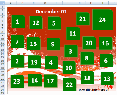
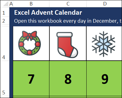
The calendar is in a 6 x 4 grid of cells, numbered from 1 to 24. Each day, the next number changes to a picture automatically – you don't have to click anything.
日历位于6 x 4的单元格网格中,从1到24编号。每天,下一个数字会自动更改为图片-您无需单击任何内容。
创建背景图片 (Create a Background Picture)
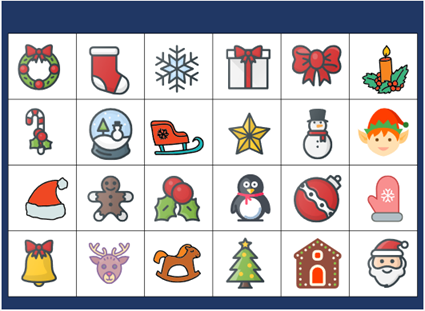
Instead of using a random layout for the pictures, I created an image with the Advent calendar "treats" carefully lined up.
我没有为图片使用随机布局,而是创建了仔细排列了Advent日历“处理”的图像。
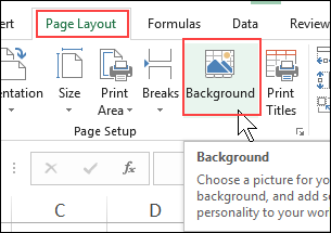
If you put an image on a worksheet, it's on top of the cells, and covers everything up. I needed the image behind the cells, for this no-macro Excel Advent calendar to work.
如果将图像放在工作表上,则它位于单元格的顶部,并且覆盖了所有内容。 我需要单元格后面的图像,才能使此无宏的Excel Advent日历正常工作。
So, instead of inserting the image on the sheet, I went to the Page Layout tab on the Excel Ribbon, and click the Background command. Then I selected my calendar grid image to use as the worksheet's background.
因此,我没有在表格上插入图像,而是转到Excel功能区上的“页面布局”选项卡,然后单击“背景”命令。 然后,我选择了日历网格图像作为工作表的背景。
涵盖背景 (Cover the Background)
When you add a Background image, you don't just get one copy of it. No, you get an entire worksheet with the image repeated!
添加背景图像时,您不仅会得到一个副本。 不,您将获得一张完整的工作表,其中包含重复的图像!
To fix that problem, and end up with only one visible image, I followed these steps:
为了解决该问题,并仅获得一张可见图像,我按照以下步骤操作:
- First, adjust the column and row widths for the 6 x 4 grid, to line up with the grid in the background image 首先,调整6 x 4网格的列和行宽度,使其与背景图像中的网格对齐
- Then, select all the cells, and use a fill colour to cover the background (I used dark blue) 然后,选择所有单元格,并使用填充色覆盖背景(我使用了深蓝色)
- Finally, select the cells in the 6 x 4 grid, and change them to No Fill 最后,在6 x 4网格中选择单元格,并将其更改为“无填充”
Admin_Dates工作表 (Admin_Dates Sheet)
There's another sheet in the Advent Calendar workbook – Admin_Dates. It helps with the formatting and formulas.
在Advent日历工作簿中还有另一个工作表– Admin_Dates。 它有助于格式和公式。
At the top of the sheet, there are formulas to calculate the current day and month, and yellow cells where you can enter a different date, for testing.
在表格的顶部,有一些公式可以计算当前的日期和月份,还有可以输入不同日期进行测试的黄色单元格。
Three of the cells are named:
其中三个单元名为 :
- Cell C2 is named CurrMth 单元格C2命名为CurrMth
- D2 is named CurrDay D2命名为CurrDay
- F2 is named AdvMth F2被命名为AdvMth
There is also a 6x4 grid with numbers for the Calendar sheet.
还有一个6x4网格,其中有用于“日历”工作表的数字。
加数字 (Add the Numbers)
The Advent calendar has 24 doors (cells). Each door should show a number, until its day arrives. After that, it should show a Christmas picture.
降临日历有24个门(单元)。 每扇门应该显示一个数字,直到它的一天到来。 之后,它应该显示圣诞节图片。
To make the numbers stand out, I used Calibri, Bold, 36, centred horizontally and vertically.
为了使数字突出,我使用了Calibri,Bold(36岁),水平和垂直居中。
To show or hide the number without macros, I used a formula in each cell, linking to the 6x4 grid on the Admin_Dates sheet.
为了显示或隐藏没有宏的数字,我在每个单元格中使用了一个公式,链接到Admin_Dates工作表上的6x4网格。
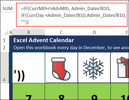
Here is the formula from cell B4, the first cell in the Advent Calendar grid. It refers to cell B10 on the Admin_Dates sheet, where the Days Grid starts.
这是单元格B4中的公式,单元格B4是“出现日历”网格中的第一个单元格。 它引用“天数网格”开始的Admin_Dates表上的单元格B10。
=IF(CurrMth<>AdvMth, Admin_Dates!B10, IF(CurrDay <Admin_Dates!B10, Admin_Dates!B10, ""))
= IF(CurrMth <> AdvMth,Admin_Dates!B10,IF(CurrDay <Admin_Dates!B10,Admin_Dates!B10,“”))
- If the current month isn't December (AdvMth=12), show the cell's number, from the reference grid on the Admin_Dates sheet. 如果当前月份不是12月(AdvMth = 12),请从Admin_Dates工作表上的参考网格中显示单元格的编号。
- If the current day number is less than then day number in the reference grid, show the cell's number 如果当前天数小于参考网格中的天数,请显示单元格的数字
- Otherwise, show an empty string (""), so we can see the picture. 否则,请显示一个空字符串(“”),以便我们可以看到图片。
添加条件格式 (Add Conditional Formatting)
You should only be able to see the Advent calendar "treats" when you reach that day of the month. Before that, the picture should be hidden.
当您到达某个月份的那天时,您应该只能看到Advent日历“治疗”。 在此之前,图片应该被隐藏。
The calendar grid has No Fill, and I added Conditional Formatting to show a green fill colour, when the cell contains a number.
日历网格没有填充,并且当单元格包含数字时,我添加了条件格式以显示绿色填充颜色。
To add the conditional formatting:
要添加条件格式:
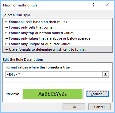
- Select cell B4:G7 (the calendar grid cells) 选择单元格B4:G7(日历网格单元格)
- On the Home tab of the Excel Ribbon, click Conditional Formatting, and click New Rule 在Excel功能区的“主页”选项卡上,单击“条件格式”,然后单击“新建规则”
- In the Select a Rule Type section, choose Use a Formula to determine which cells to format 在“选择规则类型”部分中,选择“使用公式来确定要格式化的单元格”
In the formula box, type this rule, referring to the active cell (B4): =B4<>""
在公式框中,键入以下规则,以引用活动单元格(B4): = B4 <>“”
- Click the Format button, and on the Fill tab, choose Green as the fill colour. 单击格式按钮,然后在填充选项卡上,选择绿色作为填充色。
- Click OK, twice, to apply the Conditional Format 单击确定两次,以应用条件格式
The formula checks the cell, to see if it contains an empty string. If not, the conditional formatting will be applied, and the cell will have green fill.
该公式检查单元格,以查看其是否包含空字符串。 否则,将应用条件格式,并且单元格将显示为绿色。
背景图片 (The Background Image)
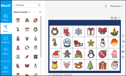
Here's how I made the image for the background, in case you're interested.
如果您有兴趣,这是我为背景制作图像的方法。
- First, I set up the worksheet, with the heading rows, and the calendar grid cells the approximate size that I wanted them. 首先,设置工作表,其中包含标题行,以及日历网格单元格所需的近似大小。
- Next, I took a screen shot with Snagit, and checked its size in Windows Explorer. 接下来,我使用Snagit进行了屏幕截图,并在Windows资源管理器中检查了它的大小。
Then I uploaded that screen shot to Stencil, which I use to make graphics.
然后,我将该屏幕快照上传到了Stencil,用于制作图形 。
- I made a new image, with my screen shot as a background, set for its size 我以屏幕截图为背景制作了一个新图像,并为其设置了大小
- Then I searched for Christmas icons, and put one into each square, resizing each one to fit. 然后,我搜索了圣诞节图标,并在每个正方形中放了一个,然后将每个大小调整为适合的大小。
- Finally, I downloaded the image in png format, to keep it as small as possible. 最后,我下载了png格式的图片,以使其尽可能小。
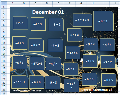
WingDings降临日历 (The WingDings Advent Calendar)
If that background image Excel Advent calendar is too fancy for you, there's good news! I made another no-macros Advent Calendar this year, and it's an even smaller, plainer file. Instead of a background picture, the "treats" are created with a font.
如果该背景图像Excel Advent日历对您来说太花哨了,那么有个好消息! 我今年又制作了一个无宏观出现的日历,这是一个更小,更简单的文件。 代替背景图片,而是使用字体创建“处理”。
The main page uses Wingdings font, because it has both numbers and pictures. (WingDings 2 is similar). And yes, most of the images are from the 1950s, but your kids will have fun guessing what they are!
主页使用Wingdings字体,因为它既包含数字又包含图片。 (WingDings 2与此类似)。 是的,大多数图像来自1950年代,但是您的孩子会很有趣地猜测它们是什么!
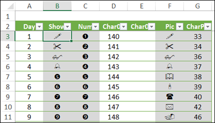
On another sheet, the CHAR Function pulls the number and picture options for each square, based on the character numbers. This formula is in cell C3, to create the one or two digit number.
在另一张纸上, CHAR功能根据字符编号为每个方块拉出编号和图片选项。 此公式在单元格C3中,以创建一个或两位数字。
=CHAR(D3)&IFERROR(CHAR(E3),"")
= CHAR(D3)&IFERROR(CHAR(E3),“”)
Then, the calendar shows the number or picture, depending on the current date. This formula is in cell B3, the Show column.
然后,日历将显示数字或图片,具体取决于当前日期。 此公式在B3单元的“显示”列中。
=IF(CurrMth<>AdvMth,[@Num],IF(CurrDay<A3,[@Num],[@Pic]))
= IF(CurrMth <> AdvMth,[@ Num],IF(CurrDay <A3,[@ Num],[@ Pic])))
- If the current month (CurrMth) is not 12 (AdvMth), result is number from column C (@Num) 如果当前月份(CurrMth)不是12(AdvMth),则结果为C列中的数字(@Num)
- If the current day (CurrDay) is less than the value in column A, result is number from column C (@Num) 如果当前日期(CurrDay)小于A列中的值,则结果为C列中的数字(@Num)
- Otherwise, result is picture from column F (@Pic) 否则,结果是来自F列的图片(@Pic)
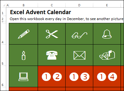
Excel Advent日历下载 (Excel Advent Calendar Downloads)
To get these Excel Advent Calendars, and see how they work, go to the Excel Advent Calendar page on my Contextures site.
要获取这些Excel Advent日历并查看其工作原理,请转到Contextures网站上的Excel Advent Calendar页面 。
That page has download links for these "no macros" Advent calendars, and for the previous versions, which do have macros.
该页面具有这些“无宏” Advent日历以及具有宏的以前版本的下载链接。
Even if you don't need an Advent calendar, you might find some useful techniques for your other Excel projects
即使您不需要Advent日历,也可能会为其他Excel项目找到一些有用的技术
翻译自: https://contexturesblog.com/archives/2018/11/29/excel-advent-calendar-no-macros/


 1425
1425

 被折叠的 条评论
为什么被折叠?
被折叠的 条评论
为什么被折叠?
 到【灌水乐园】发言


