


 这段代码展示了使用Goatlas进行的半导体器件仿真,涉及电场分布、正向与反向扫描操作,以及计算得到的反向击穿电压。代码提供了设备性能模拟的关键步骤和输出结果。
仿真代码:
go atlas

mesh  space.mult=1.0

x.mesh loc=0.00 spac=2
x.mesh loc=10.00 spac=1
x.mesh loc=40.00 spac=1
x.mesh loc=50.00 spac=2
#
y.mesh loc=-0.3 spac=0.02
y.mesh loc=0.00 spac=0.05
y.mesh loc=10.00 spac=0.5
y.mesh loc=60.00 spac=2

region   num=1 material=air y.min=-0.3 y.max=0
region   num=2 user.material=Ga2O3 y.min=0 y.max=10.00
region   num=3 user.material=Ga2O3 y.min=10.00 y.max=60
region   num=4 material=Nickel y.min=-0.3 y.max=0 x.min=10.00 x.max=40.00

electr reg=4 name=anode
electr name=cathode  bot

#....   N-epi doping
doping  region=2 n.type conc=5e16 uniform

#....   N+ doping
doping  region=3 n.type conc=1e18 uniform

material material=Ga2O3 user.default=GaN user.group=semiconductor \
         affinity=4.0 eg300=4.8 nc300=3.72e18 nv300=3.72e18 permittivity=10.0  \
         taun0=1e-9 taup0=2.1e-10 mun=118 mup=50 tcon.const tc.const=0.13 \
	     NSRHN=3.0e17 NSRHP=3.0e17

models SRH fldmob  Auger print
impact selb AN1=2.5e8 AN2=2.5e8 BN1=2.26e7 BN2=2.26e7 AP1=2.23e8 AP2=2.23e8 BP1=2.7e8 BP2=2.7e8

contact  name=anode workf=4.8 surf.rec barrier

solve      init
method newton trap maxtrap=30
# 反向扫描
log outfile = sbd_Reverse.log
solve vanode=0
solve vstep=-5 vfinal=-1000 name=anode
log off
tonyplot sbd_Reverse.log
save outf=sbd_Reverse.str
tonyplot sbd_Reverse.str

output   con.band val.band flowline ex.field

solve      init
# 正向扫描
log   outf=sbd_Forward.log
solve      vanode=0.05 vstep=0.1 vfinal=2  name=anode
log off
tonyplot sbd_Forward.log
save outf=sbd_Forward.str
tonyplot sbd_Forward.str

quit
仿真结果
下图是器件的电场分布图,可以看到明显的电场集中效应


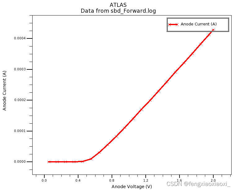
下图是器件的正向扫描曲线:
下图是器件反向扫描曲线,可以看到器件的反向击穿电压大概为327V

上述代码仅供参考,欢迎交流讨论!


 1万+
1万+

 被折叠的 条评论
为什么被折叠?
被折叠的 条评论
为什么被折叠?
 到【灌水乐园】发言


