NeRF模型之Instant-NGP原理及代码学习

最新推荐文章于 2024-04-17 10:03:31 发布

fisherisfish

最新推荐文章于 2024-04-17 10:03:31 发布

阅读量5.3k

点赞数 15

文章标签：算法

本文链接：https://blog.csdn.net/fisherisfish/article/details/132038155

版权

Instant Neural Graphics Primitives with a Multiresolution Hash Encoding

具有多分辨率哈希编码的即时神经图形基元

Overview

Instant-NGP breaks NeRF training into 3 pillars and proposes improvements to each to enable real-time training of NeRFs. The 3 pillars are:

Instant-NGP将NeRF训练分为3个支柱，并提出改进建议，以实现NeRF的实时训练。三大支柱是：

An improved training and rendering algorithm via a ray marching scheme which uses an occupancy grid
A smaller, fully-fused neural network
An effective multi-resolution hash encoding, the main contribution of this paper

1.通过使用占用网格的光线行进方案改进的训练和渲染算法

2.更小的、完全融合的神经网络

3.一种有效的多分辨率哈希编码，是本文的主要贡献。

The core idea behind the improved sampling technique is that sampling over empty space should be skipped and sampling behind high density areas should also be skipped. This is achieved by maintaining a set of multiscale occupancy grids which coarsely mark empty and non-empty space. Occupancy is stored as a single bit, and a sample on a ray is skipped if its occupancy is too low. These occupancy grids are stored independently of the trainable encoding and are updated throughout training based on the updated density predictions. The authors find they can increase sampling speed by 10-100x compared to naive approaches.

改进的采样技术背后的核心思想是，应该跳过空白区域的采样，也应该跳过高密度区域后面的采样。这是通过维护一组多尺度占用网格来实现的，这些网格粗略地标记空空间和非空空间。占用率存储为单个位，如果占用率太低，则跳过射线上的样本。这些占用网格独立于可训练编码进行存储，并在整个训练过程中根据更新的密度预测进行更新。作者发现，与朴素的方法相比，它们可以将采样速度提高 10-100 倍。

Another major bottleneck for NeRF’s training speed has been querying the neural network. The authors of this work implement the network such that it runs entirely on a single CUDA kernel. The network is also shrunk down to be just 4 layers with 64 neurons in each layer. They show that their fully-fused neural network is 5-10x faster than a Tensorflow implementation.

NeRF训练速度的另一个主要瓶颈是查询神经网络。这项工作的作者实现了网络，使其完全在单个 CUDA 内核上运行。网络也缩小到只有4层，每层有64个神经元。他们表明，他们的完全融合神经网络比Tensorflow实现快5-10倍。

The speedups at each level are multiplicative. With all their improvements, Instant-NGP reaches speedups of 1000x, which enable training NeRF scenes in a matter of seconds!

每个级别的加速是乘法的。通过所有改进，Instant-NGP 达到了 1000 倍的加速，可以在几秒钟内训练 NeRF 场景！

Multi-Resolution Hash Encoding

One contribution of Instant-NGP is the multi-resolution hash encoding. In the traditional NeRF pipelines, input coordinates are mapped to a higher dimensional space using a positional encoding function, which is described here. Instant-NGP proposes a trainable hash-based encoding. The idea is to map coordinates to trainable feature vectors which can be optimized in the standard flow of NeRF training.

Instant-NGP的一个贡献是多分辨率哈希编码。在传统的NeRF pipeline中，输入坐标使用位置编码函数映射到更高维的空间，如下所述。Instant-NGP提出了一种可训练的基于哈希的编码。这个想法是将坐标映射到可训练的特征向量，这些特征向量可以在NeRF训练的标准流程中进行优化。

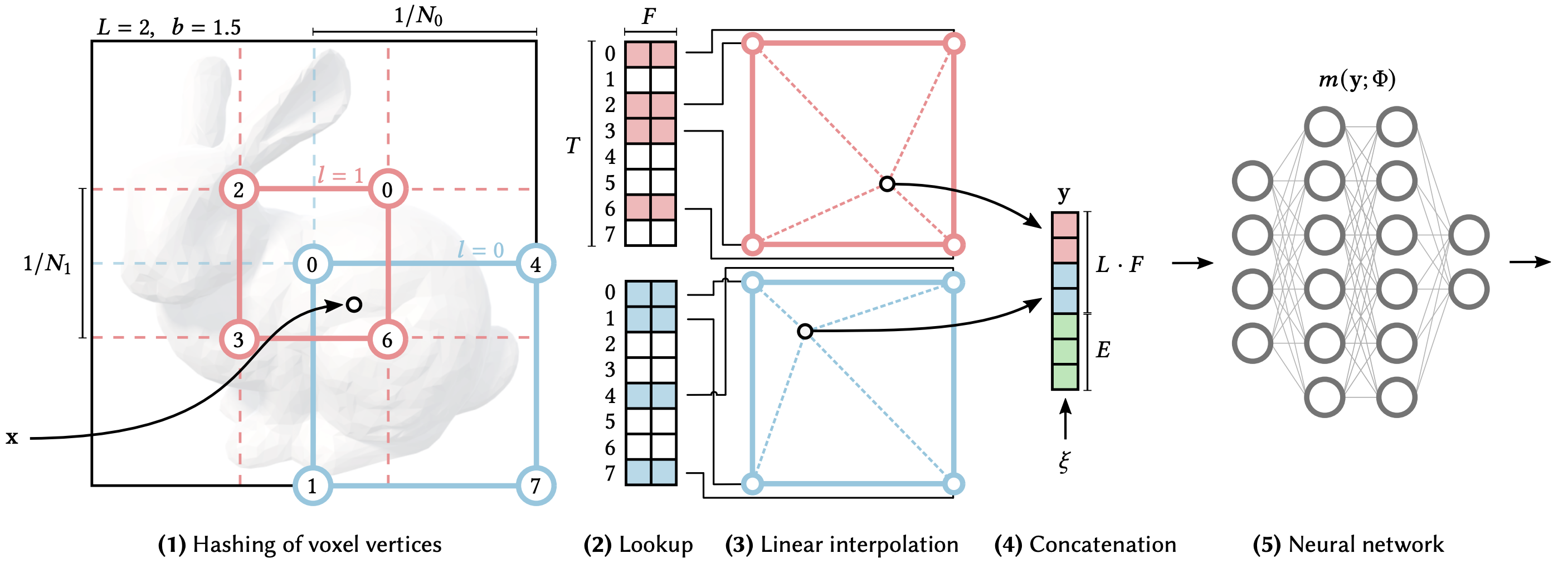
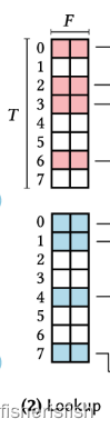
The trainable features are F-dimensional vectors and are arranged into L grids which contain up to T vectors, where L represents the number of resolutions for features and T represents the number of feature vectors in each hash grid. The steps for the hash grid encoding, as shown in the figure provided by the authors, are as follows:

可训练特征是 F 维向量，排列成最多包含 T 向量的 L 网格，其中 L 表示特征的分辨率数，T 表示每个哈希网格中的特征向量数。哈希网格编码的步骤，如图作者提供的图所示，如下所示：

../../_images/hash_figure.png

Given an input coordinate, find the surrounding voxels at L resolution levels and hash the vertices of these grids.
The hashed vertices are used as keys to look up trainable F-dimensional feature vectors.
Based on where the coordinate lies in space, the feature vectors are linearly interpolated to match the input coordinate.
The feature vectors from each grid are concatenated, along with any other parameters such as viewing direction,
The final vector is inputted into the neural network to predict the RGB and density output.

1、给定输入坐标，在 L 分辨率级别查找周围的体素并对这些格网的顶点进行哈希处理。

2、散列顶点用作查找可训练 F 维特征向量的键。

3、根据坐标在空间中的位置，对要素向量进行线性插值以匹配输入坐标。

4、连接来自每个网格的特征向量以及任何其他参数，例如查看方向

5、最终向量被输入神经网络以预测RGB和密度输出。

Steps 1-3 are done independently at each resolution level. Thus, since these feature vectors are trainable, when backpropagating the loss gradient, the gradients will flow through the neural network and interpolation function all the way back to the feature vectors. The feature vectors are interpolated relative to the coordinate such that the network can learn a smooth function.

步骤 1-3 在每个分辨率级别独立完成。因此，由于这些特征向量是可训练的，当反向传播损失梯度时，梯度将通过神经网络和插值函数一直流回特征向量。特征向量相对于坐标进行插值，以便网络可以学习平滑函数。

An important note is that hash collisions are not explicitly handled. At each hash index, there may be multiple vertices which index to that feature vector, but because these vectors are trainable, the vertices that are most important to the specific output will have the highest gradient, and therefore automatically dominate the optimization of that feature.

一个重要的注意事项是，哈希冲突没有显式处理。在每个哈希索引中，可能有多个顶点索引到该特征向量，但由于这些向量是可训练的，因此对特定输出最重要的顶点将具有最高的梯度，因此自动主导该特征的优化。

This encoding structure creates a tradeoff between quality, memory, and performance. The main parameters which can be adjusted are the size of the hash table (T), the size of the feature vectors (F), and the number of resolutions (L).

这种编码结构在质量、内存和性能之间进行了权衡。可以调整的主要参数是哈希表的大小（T），特征向量的大小（F）和分辨率的数量（L）。

Instant-NGP encodes the viewing direction using spherical harmonic encodings.

Instant-NGP 使用spherical harmonic encodings对viewing direction进行编码。

上文是NeRFStudio中对InstantNGP模型的介绍，经过学习可以知道InstantNGP最核心的改进在于两点，一点就是Multi-Resolution Hash Encoding，另一点则是基于cuda编程的MLP模型。

从实验上来看确实效果很好，在本人的4060笔记本上InstantNGP大约10s就能渲染出一个场景，这里研究一下其原理和代码实现。虽然但是我没想到官方直接给了应用程序，而且实现是基于cuda的，要学习的内容有点多，但我会尽力一点一点掰开来看的。

好消息是有大佬用pytorch实现了，我计划先用pytorch版本理解具体流程，然后再看cuda版本的实现学习cuda。yysy，NeRF讲解得还挺多的，这个讲解反而比较少，也算是一项开创性的工作吧。

GitHub - yashbhalgat/HashNeRF-pytorch: Pure PyTorch Implementation of NVIDIA paper on Instant Training of Neural Graphics primitives: https://nvlabs.github.io/instant-ngp/

Multi-Resolution Hash Encoding其实是对NeRF中的线性编码的一种优化，首先先看HashEmbedder的输入。

def get_embedder(multires, args, i=0):
    if i == -1:
        return nn.Identity(), 3
    elif i==0:
        embed_kwargs = {
                    'include_input' : True,
                    'input_dims' : 3,
                    'max_freq_log2' : multires-1,
                    'num_freqs' : multires,
                    'log_sampling' : True,
                    'periodic_fns' : [torch.sin, torch.cos],
        }
        
        embedder_obj = Embedder(**embed_kwargs)
        embed = lambda x, eo=embedder_obj : eo.embed(x)
        out_dim = embedder_obj.out_dim
    elif i==1:
        embed = HashEmbedder(bounding_box=args.bounding_box, \
                            log2_hashmap_size=args.log2_hashmap_size, \
                            finest_resolution=args.finest_res)
        out_dim = embed.out_dim
    elif i==2:
        embed = SHEncoder()
        out_dim = embed.out_dim
    return embed, out_dim

bounding_box来自于读取数据时的输入，在load_blender函数中，

    bounding_box = get_bbox3d_for_blenderobj(metas["train"], H, W, near=2.0, far=6.0)


def get_bbox3d_for_blenderobj(camera_transforms, H, W, near=2.0, far=6.0):

    //获取相机水平视场 (horizontal field of view)，用于计算焦距 (focal)
    camera_angle_x = float(camera_transforms['camera_angle_x'])
    focal = 0.5*W/np.tan(0.5 * camera_angle_x)

    # ray directions in camera coordinates
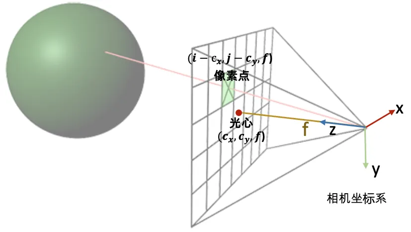
    //就是get_rays函数，但是只提取方向，顺便复习一下光线方向如何计算得到，值得一提的是此处的射线方式是处在相机坐标系下的，如果要得到世界坐标系下的射线方向需要c2w*rays_d
    directions = get_ray_directions(H, W, focal)

//
def get_ray_directions(H, W, focal):
    """
    Get ray directions for all pixels in camera coordinate.
    Reference: https://www.scratchapixel.com/lessons/3d-basic-rendering/
               ray-tracing-generating-camera-rays/standard-coordinate-systems

    Inputs:
        H, W, focal: image height, width and focal length

    Outputs:
        directions: (H, W, 3), the direction of the rays in camera coordinate
    """
    grid = create_meshgrid(H, W, normalized_coordinates=False)[0]
    i, j = grid.unbind(-1)
    # the direction here is without +0.5 pixel centering as calibration is not so accurate
    # see https://github.com/bmild/nerf/issues/24
    directions = \
        torch.stack([(i-W/2)/focal, -(j-H/2)/focal, -torch.ones_like(i)], -1) # (H, W, 3)

    dir_bounds = directions.view(-1, 3)
    # print("Directions ", directions[0,0,:], directions[H-1,0,:], directions[0,W-1,:], directions[H-1, W-1, :])
    # print("Directions ", dir_bounds[0], dir_bounds[W-1], dir_bounds[H*W-W], dir_bounds[H*W-1])

    return directions
//

    //这里定义了一个最小和最大的bound，即所有点的最小边界和最大边界，所有点都会在这两个边界之间
    min_bound = [100, 100, 100]
    max_bound = [-100, -100, -100]

    points = []

    for frame in camera_transforms["frames"]:
        //逐帧获取图像的外参，进行射线计算
        c2w = torch.FloatTensor(frame["transform_matrix"])
        rays_o, rays_d = get_rays(directions, c2w)
        

//
def get_rays(directions, c2w):
    """
    Get ray origin and normalized directions in world coordinate for all pixels in one image.
    Reference: https://www.scratchapixel.com/lessons/3d-basic-rendering/
               ray-tracing-generating-camera-rays/standard-coordinate-systems

    Inputs:
        directions: (H, W, 3) precomputed ray directions in camera coordinate
        c2w: (3, 4) transformation matrix from camera coordinate to world coordinate

    Outputs:
        rays_o: (H*W, 3), the origin of the rays in world coordinate
        rays_d: (H*W, 3), the normalized direction of the rays in world coordinate
    """
    # Rotate ray directions from camera coordinate to the world coordinate
    //即c2w*rays_d最后结果和原nerf中的rays_d = torch.sum(directions[..., np.newaxis, :] * c2w[:3, :3], -1)相同，但这个式子容易理解了许多
    rays_d = directions @ c2w[:3, :3].T # (H, W, 3)
    //归一化操作
    rays_d = rays_d / torch.norm(rays_d, dim=-1, keepdim=True)
    # The origin of all rays is the camera origin in world coordinate
    //c2w矩阵中的最后一列即为世界坐标系下的相机坐标
    rays_o = c2w[:3, -1].expand(rays_d.shape) # (H, W, 3)

    rays_d = rays_d.view(-1, 3)
    rays_o = rays_o.view(-1, 3)

    return rays_o, rays_d
//
        //寻找最大最小的包围框，针对射线上的点
        def find_min_max(pt):
            for i in range(3):
                if(min_bound[i] > pt[i]):
                    min_bound[i] = pt[i]
                if(max_bound[i] < pt[i]):
                    max_bound[i] = pt[i]
            return
        
        //循环取射线，但是每帧只取0，399，159600，159999的射线即上下左右四条射线，min_bound和max_bound将不断更新为包含这光线上最小点和最大点的两个矩阵，以lego为例，最后的min_bound:[tensor(-3.0182, device='cpu'), tensor(-3.0058, device='cpu'), tensor(-2.3284, device='cpu')]
max_bound:[tensor(3.0072, device='cpu'), tensor(3.0174, device='cpu'), tensor(2.3384, device='cpu')]
        for i in [0, W-1, H*W-W, H*W-1]:
            min_point = rays_o[i] + near*rays_d[i]
            max_point = rays_o[i] + far*rays_d[i]
            points += [min_point, max_point]
            find_min_max(min_point)
            find_min_max(max_point)
    //return这里为啥要减和加呢？我个人理解是为了保证这个bounding能包含所有点做的一步扩充
    return (torch.tensor(min_bound)-torch.tensor([1.0,1.0,1.0]), torch.tensor(max_bound)+torch.tensor([1.0,1.0,1.0]))

log2_hashmap_size是args的输入，默认是19，log2 of hashmap size，即论文中的T

finest_res也是args的输入，默认是512，finest resolultion for hashed embedding，即论文中的Nmax

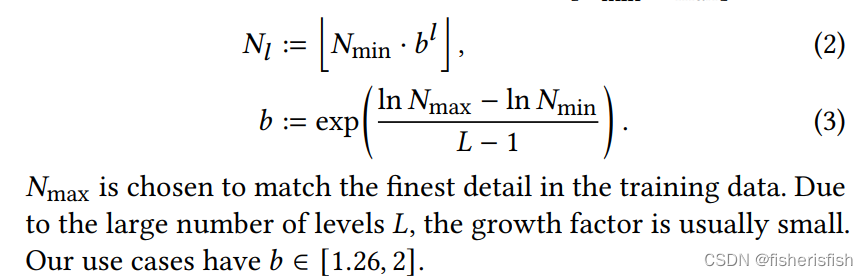
接下来是这个HashEmbedder的代码，这里参考原文的公式𝑁min=base_resolution，𝑁max=finest_resolution，其余参数含义见下表

../../_images/hash_figure.png

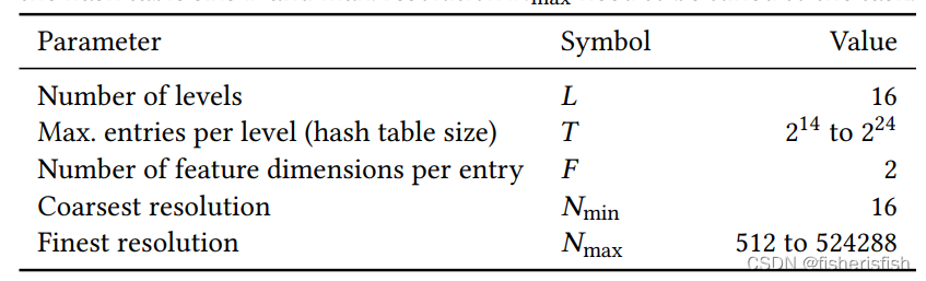
out_dim=L*F ，b的值来自于下文的公式

class HashEmbedder(nn.Module):
    def __init__(self, bounding_box, n_levels=16, n_features_per_level=2,\
                log2_hashmap_size=19, base_resolution=16, finest_resolution=512):
        super(HashEmbedder, self).__init__()
        self.bounding_box = bounding_box
        self.n_levels = n_levels
        self.n_features_per_level = n_features_per_level//F=2
        self.log2_hashmap_size = log2_hashmap_size//T=19
        self.base_resolution = torch.tensor(base_resolution)
        self.finest_resolution = torch.tensor(finest_resolution)
        self.out_dim = self.n_levels * self.n_features_per_level

        self.b = torch.exp((torch.log(self.finest_resolution)-torch.log(self.base_resolution))/(n_levels-1))

torch.nn.Embedding(numembeddings,embeddingdim)的意思是创建一个词嵌入模型，numembeddings代表一共有多少个词, embedding_dim代表你想要为每个词创建一个多少维的向量来表示它，nn.ModuleList代表产生了16个这样的nn.Embedding层，nn.init.uniform_对值进行初始化，torch.nn.init.uniform_(tensor, a=0, b=1)，均匀分布，服从~U(a,b)U(a, b)U(a,b)

        self.embeddings = nn.ModuleList([nn.Embedding(2**self.log2_hashmap_size, \
                                        self.n_features_per_level) for i in range(n_levels)])

//
ModuleList(
  (0): Embedding(524288, 2)
  (1): Embedding(524288, 2)
  (2): Embedding(524288, 2)
  (3): Embedding(524288, 2)
  (4): Embedding(524288, 2)
  (5): Embedding(524288, 2)
  (6): Embedding(524288, 2)
  (7): Embedding(524288, 2)
  (8): Embedding(524288, 2)
  (9): Embedding(524288, 2)
  (10): Embedding(524288, 2)
  (11): Embedding(524288, 2)
  (12): Embedding(524288, 2)
  (13): Embedding(524288, 2)
  (14): Embedding(524288, 2)
  (15): Embedding(524288, 2)
)
//

        # custom uniform initialization
        for i in range(n_levels):
            nn.init.uniform_(self.embeddings[i].weight, a=-0.0001, b=0.0001)
            # self.embeddings[i].weight.data.zero_()

Embedding的具体含义可以见下图，2**19的hash table对应长度为2的特征，需要反馈训练得到，来解决hash冲突。

接下来我们来看一下前向推理的过程，embedding的输入在原nerf中有xyz和方位视角（θ，φ）两类，而在instantNGP中hashembedding的输入为xyz，方位视角（θ，φ）则采用了SHEncoder，这两个输入值xyz为各个射线上的采样点坐标得到，方位视角（θ，φ）即归一化后的rays_d向量也叫viewdirs 。其实在论文中InstantNGP似乎是采用了一种不同的采样点策略，但在这个Pytorch版本里和NeRF采样策略是一样的，从近端到远端平均采64个点，再加上从图像中随机取1024个点，所以最后的hashembedding输入就是[1024*64,3]，代表着图像上1024个随机点的射线上64个采样点的坐标。

中间层的resolution计算公式如论文中的公式2，然后是这个比较关键的get_voxel_vertices，函数的输入有x即输入的xyz坐标，bounding_box即所有射线的包围框，resolution和log2_hashmap_size即论文中T的值。

    def forward(self, x):
        # x is 3D point position: B x 3
        x_embedded_all = []
        for i in range(self.n_levels):
            resolution = torch.floor(self.base_resolution * self.b**i)
            voxel_min_vertex, voxel_max_vertex, hashed_voxel_indices, keep_mask = get_voxel_vertices(\
                                                x, self.bounding_box, \
                                                resolution, self.log2_hashmap_size)

keep_mask这部是检查点是否是在包围框内的？后续还有一步也是这个作用，grid的数量即resolution，grid_size即大小，作为一个hash表学得不好的人，实在是很难理解这一部分，只能靠论文和自己理解一步步走，

grid_size = (box_max-box_min)/resolution //三边长除以分辨率
bottom_left_idx = torch.floor((xyz-box_min)/grid_size).int()//获取点在哪个网格中的坐标信息，即点所在grid的index，包括xyz三个维度[65536,3]

voxel_min_vertex = bottom_left_idx*grid_size + box_min
voxel_max_vertex = voxel_min_vertex + torch.tensor([1.0,1.0,1.0])*grid_size

这两句是计算点所在voxel的空间最大和最小顶点坐标值

voxel_indices = bottom_left_idx.unsqueeze(1) + BOX_OFFSETS//当前点位对应四周八个点位的index，[65536,8,3]
hashed_voxel_indices = hash(voxel_indices, log2_hashmap_size)

def get_voxel_vertices(xyz, bounding_box, resolution, log2_hashmap_size):
    '''
    xyz: 3D coordinates of samples. B x 3
    bounding_box: min and max x,y,z coordinates of object bbox
    resolution: number of voxels per axis
    '''
    box_min, box_max = bounding_box

    keep_mask = xyz==torch.max(torch.min(xyz, box_max), box_min)
    if not torch.all(xyz <= box_max) or not torch.all(xyz >= box_min):
        # print("ALERT: some points are outside bounding box. Clipping them!")
        xyz = torch.clamp(xyz, min=box_min, max=box_max)

    grid_size = (box_max-box_min)/resolution
    
    bottom_left_idx = torch.floor((xyz-box_min)/grid_size).int()
    voxel_min_vertex = bottom_left_idx*grid_size + box_min
    voxel_max_vertex = voxel_min_vertex + torch.tensor([1.0,1.0,1.0])*grid_size

    voxel_indices = bottom_left_idx.unsqueeze(1) + BOX_OFFSETS
    hashed_voxel_indices = hash(voxel_indices, log2_hashmap_size)

    //返回值为voxel最小点最大点的空间坐标，以及八个点的hashtable下标值
    return voxel_min_vertex, voxel_max_vertex, hashed_voxel_indices, keep_mask

primes即论文中的Πi,为随机取得大质数，由于xi只有xyz三个值，所以只用到前三个值，hash函数的输入即点所在voxel的八个坐标点的index，xor为按位异或运算

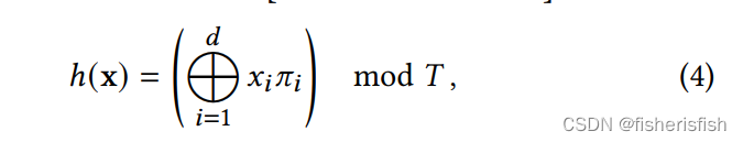
def hash(coords, log2_hashmap_size):
    '''
    coords: this function can process upto 7 dim coordinates
    log2T:  logarithm of T w.r.t 2
    '''
    //只用到前三个
    primes = [1, 2654435761, 805459861, 3674653429, 2097192037, 1434869437, 2165219737]

    xor_result = torch.zeros_like(coords)[..., 0]
    for i in range(coords.shape[-1]):
        //最后一个维度，即取index的坐标xyz
        //0 ^ index[0]*1 ^ index[1]*2654435761 ^ index[2]*805459861
        xor_result ^= coords[..., i]*primes[i]

    //和T取模，最终返回八个点在hash table中的下标
    return torch.tensor((1<<log2_hashmap_size)-1).to(xor_result.device) & xor_result

trilinear_interp为三维线性插值函数，根据voxel的点坐标计算x点的坐标并返回x的特征向量，由于总共有16层这样的embedding，所以最后的输出大小为[65536,16*2]

            
            //根据hash table索引获得八个点的特征[65536,8,2]
            voxel_embedds = self.embeddings[i](hashed_voxel_indices)
            //输出大小为[65536,2]
            x_embedded = self.trilinear_interp(x, voxel_min_vertex, voxel_max_vertex, voxel_embedds)
            x_embedded_all.append(x_embedded)

    def trilinear_interp(self, x, voxel_min_vertex, voxel_max_vertex, voxel_embedds):
        '''
        x: B x 3
        voxel_min_vertex: B x 3
        voxel_max_vertex: B x 3
        voxel_embedds: B x 8 x 2
        '''
        # source: https://en.wikipedia.org/wiki/Trilinear_interpolation
        weights = (x - voxel_min_vertex)/(voxel_max_vertex-voxel_min_vertex) # B x 3

        # step 1
        # 0->000, 1->001, 2->010, 3->011, 4->100, 5->101, 6->110, 7->111
        c00 = voxel_embedds[:,0]*(1-weights[:,0][:,None]) + voxel_embedds[:,4]*weights[:,0][:,None]
        c01 = voxel_embedds[:,1]*(1-weights[:,0][:,None]) + voxel_embedds[:,5]*weights[:,0][:,None]
        c10 = voxel_embedds[:,2]*(1-weights[:,0][:,None]) + voxel_embedds[:,6]*weights[:,0][:,None]
        c11 = voxel_embedds[:,3]*(1-weights[:,0][:,None]) + voxel_embedds[:,7]*weights[:,0][:,None]

        # step 2
        c0 = c00*(1-weights[:,1][:,None]) + c10*weights[:,1][:,None]
        c1 = c01*(1-weights[:,1][:,None]) + c11*weights[:,1][:,None]

        # step 3
        c = c0*(1-weights[:,2][:,None]) + c1*weights[:,2][:,None]

        return c

接下来是NeRFsmall的前向推理过程，这里的输入为[65536,32+16]其中32是xyzhash编码得到的，16为方位视角（θ，φ）SHEncoder得到的，和NeRF不同的是，32作为体积密度sigma_net的输入，最后输出为16，sigma_net非常简单，32->64->16，然后取出第一个值作为sigma，后面15个值和方位视角（θ，φ）SHEncoder得到的input_views结合，color_net也非常简单，31->64->64->3，最后输出为rgb sigma组成的[65536,4]

    def forward(self, x):
        input_pts, input_views = torch.split(x, [self.input_ch, self.input_ch_views], dim=-1)

        # sigma
        h = input_pts
        for l in range(self.num_layers):
            h = self.sigma_net[l](h)
            if l != self.num_layers - 1:
                h = F.relu(h, inplace=True)

        sigma, geo_feat = h[..., 0], h[..., 1:]
        
        # color
        h = torch.cat([input_views, geo_feat], dim=-1)
        for l in range(self.num_layers_color):
            h = self.color_net[l](h)
            if l != self.num_layers_color - 1:
                h = F.relu(h, inplace=True)
            
        # color = torch.sigmoid(h)
        color = h
        outputs = torch.cat([color, sigma.unsqueeze(dim=-1)], -1)

        return outputs

然后顺便讲一下方位角的SHEncode也就是球谐基投影。

球谐函数的介绍大佬介绍得非常好，但是我对于公式还是不了解，希望后续有大佬能介绍一下这个编码方式

球谐函数介绍（Spherical Harmonics） - 知乎 (zhihu.com)

class SHEncoder(nn.Module):
    def __init__(self, input_dim=3, degree=4):
    
        super().__init__()

        self.input_dim = input_dim
        self.degree = degree

        assert self.input_dim == 3
        assert self.degree >= 1 and self.degree <= 5

        self.out_dim = degree ** 2

        self.C0 = 0.28209479177387814
        self.C1 = 0.4886025119029199
        self.C2 = [
            1.0925484305920792,
            -1.0925484305920792,
            0.31539156525252005,
            -1.0925484305920792,
            0.5462742152960396
        ]
        self.C3 = [
            -0.5900435899266435,
            2.890611442640554,
            -0.4570457994644658,
            0.3731763325901154,
            -0.4570457994644658,
            1.445305721320277,
            -0.5900435899266435
        ]
        self.C4 = [
            2.5033429417967046,
            -1.7701307697799304,
            0.9461746957575601,
            -0.6690465435572892,
            0.10578554691520431,
            -0.6690465435572892,
            0.47308734787878004,
            -1.7701307697799304,
            0.6258357354491761
        ]

    def forward(self, input, **kwargs):

        result = torch.empty((*input.shape[:-1], self.out_dim), dtype=input.dtype, device=input.device)
        x, y, z = input.unbind(-1)

        result[..., 0] = self.C0
        if self.degree > 1:
            result[..., 1] = -self.C1 * y
            result[..., 2] = self.C1 * z
            result[..., 3] = -self.C1 * x
            if self.degree > 2:
                xx, yy, zz = x * x, y * y, z * z
                xy, yz, xz = x * y, y * z, x * z
                result[..., 4] = self.C2[0] * xy
                result[..., 5] = self.C2[1] * yz
                result[..., 6] = self.C2[2] * (2.0 * zz - xx - yy)
                #result[..., 6] = self.C2[2] * (3.0 * zz - 1) # xx + yy + zz == 1, but this will lead to different backward gradients, interesting...
                result[..., 7] = self.C2[3] * xz
                result[..., 8] = self.C2[4] * (xx - yy)
                if self.degree > 3:
                    result[..., 9] = self.C3[0] * y * (3 * xx - yy)
                    result[..., 10] = self.C3[1] * xy * z
                    result[..., 11] = self.C3[2] * y * (4 * zz - xx - yy)
                    result[..., 12] = self.C3[3] * z * (2 * zz - 3 * xx - 3 * yy)
                    result[..., 13] = self.C3[4] * x * (4 * zz - xx - yy)
                    result[..., 14] = self.C3[5] * z * (xx - yy)
                    result[..., 15] = self.C3[6] * x * (xx - 3 * yy)
                    if self.degree > 4:
                        result[..., 16] = self.C4[0] * xy * (xx - yy)
                        result[..., 17] = self.C4[1] * yz * (3 * xx - yy)
                        result[..., 18] = self.C4[2] * xy * (7 * zz - 1)
                        result[..., 19] = self.C4[3] * yz * (7 * zz - 3)
                        result[..., 20] = self.C4[4] * (zz * (35 * zz - 30) + 3)
                        result[..., 21] = self.C4[5] * xz * (7 * zz - 3)
                        result[..., 22] = self.C4[6] * (xx - yy) * (7 * zz - 1)
                        result[..., 23] = self.C4[7] * xz * (xx - 3 * yy)
                        result[..., 24] = self.C4[8] * (xx * (xx - 3 * yy) - yy * (3 * xx - yy))

        return result

NGP内容梳理完后，会先放一放三维重建，将聚焦于二维图像生成，最终的目标是实现人工手绘草图然后直接输出三维建模的流程。