[机器学习实验4]正则化（引入惩罚因子）

数据下载链接：
http://openclassroom.stanford.edu/MainFolder/courses/MachineLearning/exercises/ex5materials/ex5Data.zip
本次实验的主要目的是了解引入的正则化参数对拟合效果的影响，通过调整该参数来解决过拟合和欠拟合的问题。

线性回归中引入正则化参数。

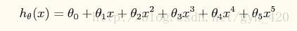
x再线性回归的实践中是一维的，如果是更高维度的还要做一个特征的转化，后面的logic回归里面会提到

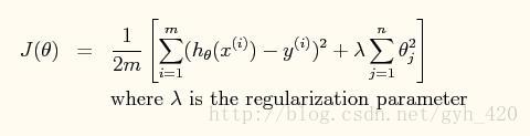
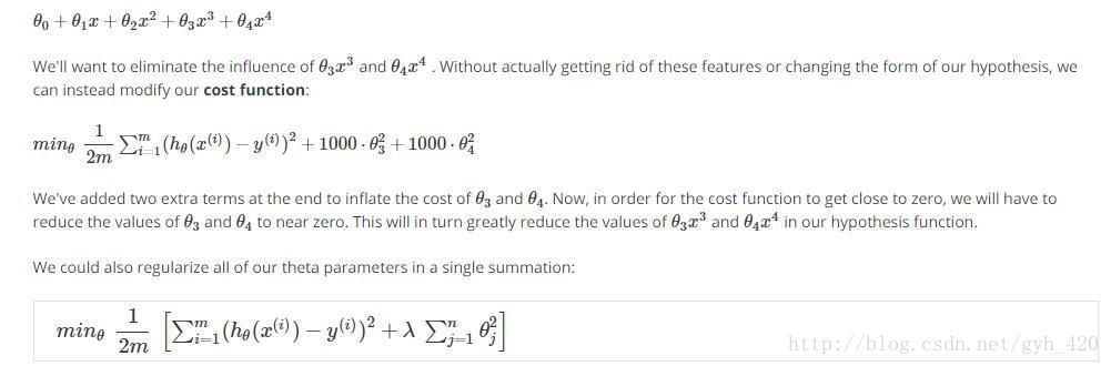
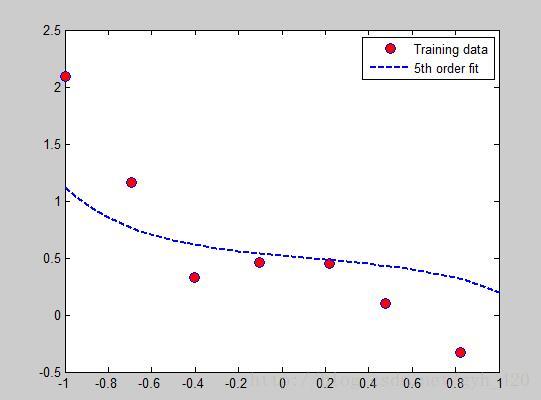
引入正则化参数之后公式如上，当最小化J(θ)时，λ 越大,θ越小，所以通过调节λ的值可以调节拟合的h函数中中θ的大小从而调节拟合的程度，λ过大会导致欠拟合，过小会导致过拟合。

为了展示出引入正则化后公式上的不同，就不实用梯度下降，实用梯度下降和之前的实验是一样的，本实验使用的是最小二乘法，公式变为：

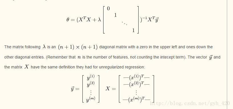
得到的θ即为我们要求的参数，通过调节λ来看拟合效果
代码如下：

%%线性回归的正则化
clear all; close all; clc
x = load('ex5Linx.dat'); y = load('ex5Liny.dat');

m = length(y); % number of training examples

% Plot the training data
figure;
plot(x, y, 'o', 'MarkerFacecolor', 'r', 'MarkerSize', 8);
% Our features are all powers of x from x^0 to x^5
x = [ones(m, 1), x, x.^2, x.^3, x.^4, x.^5];

theta = zeros(size(x(1,:)))'; % initialize fitting parameters

% The regularization parameter
lambda = 10;

% Closed form solution from normal equations
L = lambda.*eye(6); % the extra regularization terms
L(1) = 0;%theta(0)不参与

theta = (x' * x + L)\x' * y
norm_theta = norm(theta)
% Plot the linear fit
hold on;
% Our training data was only a few points, so we need
% to create a denser array of x-values for plotting
x_vals = (-1:0.05:1)';
features = [ones(size(x_vals)), x_vals, x_vals.^2, x_vals.^3,...
          x_vals.^4, x_vals.^5];
plot(x_vals, features*theta, '--', 'LineWidth', 2)
legend('Training data', '5th order fit')
hold off

λ = 10时：

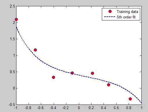
λ = 1时：

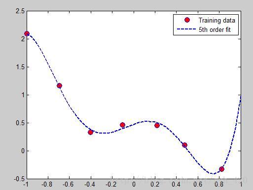
λ = 0时：

logic回归中引入正则化参数

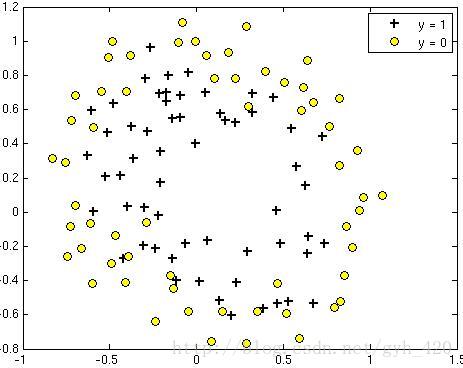
之前下载的数据集中ex5Logx，ex5Logy标记了x数据中的哪些是正（1）哪些是负（0）样本，我们拟用这个数据来训练出一个二分类器。
读取的数据如下图

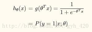
我们使用的分类函数:

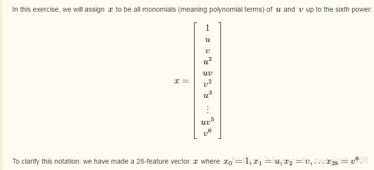
因为x的维度是二维的，就是有两个特征参数，而我们又要进行多项式拟合，那么就要扩展特征参数到高次，比如说扩展到6次方，首先还是要加入截距项（x=1的项）

代码如下：

function out = map_feature(feat1, feat2)
% MAP_FEATURE    Feature mapping function for Exercise 5
%
%   map_feature(feat1, feat2) maps the two input features
%   to higher-order features as defined in Exercise 5.
%
%   Returns a new feature array with more features
%
%   Inputs feat1, feat2 must be the same size
%
% Note: this function is only valid for Ex 5, since the degree is
% hard-coded in.
    degree = 6;
    out = ones(size(feat1(:,1)));
    for i = 1:degree
        for j = 0:i
            out(:, end+1) = (feat1.^(i-j)).*(feat2.^j);
        end
    end

更高维度的特征参数的扩展和这个方法类似，可以类推，这个部分的推导我还不是很清楚是怎么推出来的，知道的朋友可以在评论里分享出来，谢谢。
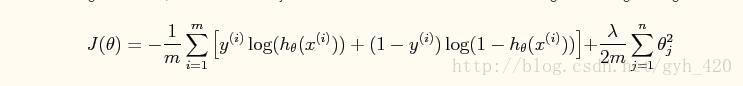
代价函数J（θ）也是类似引入惩罚项：

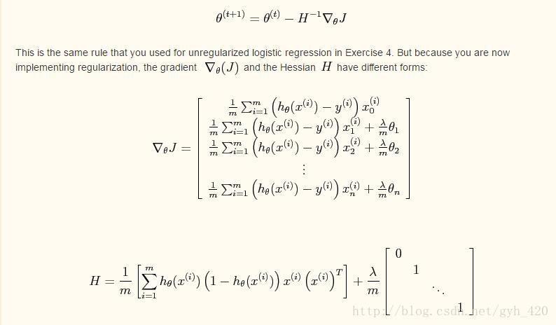
使用牛顿方法来求θ值

代码如下：

x = load('ex5Logx.dat'); 
y = load('ex5Logy.dat');

Plot the training data
Use different markers for positives and negatives
figure
pos = find(y); neg = find(y == 0);
% 正样本pos个，负样本neg个
plot(x(pos, 1), x(pos, 2), 'k+','LineWidth', 2, 'MarkerSize', 7)
hold on
plot(x(neg, 1), x(neg, 2), 'ko', 'MarkerFaceColor', 'y', 'MarkerSize', 7)

%注意这个地方的feature，x原来是一个二维的变量，一方面要插入截距（就是全为1的那列），另一方面在做非线性的拟合平面时
%它的2次方、3次方。。。n次方扩展是x1^i * x2^j这样进行的
x = map_feature(x(:,1), x(:,2));

[m, n] = size(x);

% Initialize fitting parameters
theta = zeros(n, 1);
% Define the sigmoid function
%逻辑回归的hypotheise
g = inline('1.0 ./ (1.0 + exp(-z))'); 

% setup for Newton's method
%迭代次数
MAX_ITR = 15;
J = zeros(MAX_ITR, 1);

% Lambda is the regularization parameter
lambda = 0.5;

for i = 1:MAX_ITR
    % Calculate the hypothesis function
    z = x * theta;
    h = g(z) ;%h函数

    % Calculate J (for testing convergence)
    J(i) =(1/m)*sum(-y.*log(h) - (1-y).*log(1-h))+ ...
    (lambda/(2*m))*norm(theta([2:end]))^2; %不包括theta（0）
    %norm求的是向量theta的2范数，公式中不是平方根，所以要平方一下

    % Calculate gradient and hessian.
    G = (lambda/m).*theta; G(1) = 0; % extra term for gradient
    L = (lambda/m).*eye(n); L(1) = 0;% extra term for Hessian

    %这里的两个计算和前面的logic regression实验里是一样的方法
    grad = ((1/m).*x' * (h-y)) + G;
    H = ((1/m).*x' * diag(h) * diag(1-h) * x) + L;

    % Here is the actual update
    theta = theta - H\grad;

end

% Define the ranges of the grid
u = linspace(-1, 1.5, 200);
v = linspace(-1, 1.5, 200);

% Initialize space for the values to be plotted
z = zeros(length(u), length(v));

% Evaluate z = theta*x over the grid
for i = 1:length(u)
    for j = 1:length(v)
        % Notice the order of j, i here!
        z(j,i) = map_feature(u(i), v(j))*theta;
    end
end

% Because of the way that contour plotting works
% in Matlab, we need to transpose z, or
% else the axis orientation will be flipped!
z = z'
% Plot z = 0 by specifying the range [0, 0]
contour(u,v,z, 'LineWidth', 2)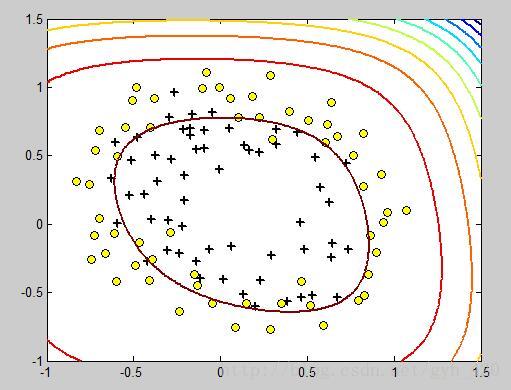

这是绘制的θ*X的方程，而我们要θ*X=0的轮廓，将
contour(u,v,z, ‘LineWidth’, 2)改成contour(u,v,z, [0,0],’LineWidth’, 2)即可

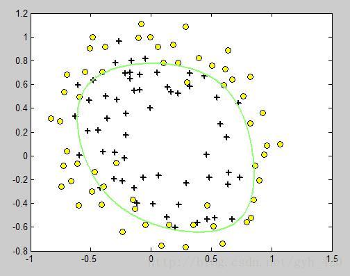
调整λ的值可以得到强弱不同的边界。