量化交易软件策略：使用计量经济学方法分析图表

简介

我经常听到有关市场动荡不稳的言论。这也解释了为何无法实现成功的长期交易。但事实果真如此吗？让我们尝试从科学的角度分析这一问题。赫兹量化将选择计量经济学方法进行分析。为何选择计量经济学方法？首先，MQL 社区热衷于追求精确性，而这只能通过数学和统计学予以实现。其次，如果我没弄错的话，之前在这方面尚属空白。

需要指出的是，成功的长期交易问题无法通过一篇文章就得以解决。现在，我只打算介绍选定模型的几种诊断方法，希望在以后的使用中能够体现其价值。

此外，我将尽可能清楚介绍一些枯燥的理论知识，包括公式、定理和假设。然而，我希望读者已经了解统计学的一些基本概念，例如：假设、统计显著性、统计（统计标准）、离差、分布、概率、回归、自相关等。

​

编辑切换为居中

添加图片注释，不超过 140 字（可选）

1. 时间序列的特性

显而易见，赫兹量化分析的对象是价格序列（及其派生物），这是一个时间序列。

计量经济学家从频率法（频谱分析、小波分析）和时域法（互相关分析、自相关分析）的角度研究时间序列。市面上已经有了频谱方法介绍方面的文章，读者可自行查阅《构建频谱分析》一文。在此，我建议将注意力集中在时域方法、自相关分析尤其是条件方差分析上。

在价格时间序列表现的描述方面，非线性模型要优于线性模型。这就是我们在本文中研究非线性模型的原因。

价格时间序列的一些特性只能通过特定的计量经济模型加以考虑。首先，这些特性包括：“肥尾”、波动集群性和杠杆效应。

​

编辑

添加图片注释，不超过 140 字（可选）

图 1. 具有不同峰度的分布。

图 1 展示了具有不同峰度（峭度）的 3 个分布。其峭度小于正态分布峭度的分布具有“肥尾”的可能性要大于其他分布。该分布标为粉红色。

赫兹量化需要分布来显示随机值的概率密度，概率密度用于计算研究序列的值。

通过提到波动的集群性（出自群集 - 群、集中），我们是指：高波动时期后会出现高波动时间周期，低波动时期后面同样会出现低波动时期。如果昨天发生价格波动，则今天也很可能发生。因此，波动存在惯性。图 2 显示波动表现为群集性。

​

编辑切换为居中

添加图片注释，不超过 140 字（可选）

图 2. USDJPY 每日收益的波动集群性。

下跌市场的波动杠杆效应要甚于上涨市场的该效应。它受制于杠杆系数的增大，而杠杆系数取决于股价下跌时所借资产与自有资产的比率。然而，该效应适用于股票市场而非期货市场。因此，赫兹量化无需对其进行更多考虑。

2. GARCH 模型

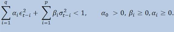
好了，赫兹量化的主要目标是通过一些模型来预测汇率（价格）。计量经济学家使用数学模型来描述可进行定量估计的某种效应。简言之，他们根据事件选用不同公式，通过这种方式来描述事件。

考虑到所分析的时间序列具有上文提到的属性，能将这些属性考虑在内的最佳模型就是非线性模型。最常用的非线性模型之一是 GARCH 模型。它将如何帮助我们？在其主体（函数）内，它将考虑序列的波动，即离差在不同观察周期的波动。计量经济学家使用了一个晦涩的术语来命名该效应 - heteroscedasticity（出自希腊语：hetero 表示“不同”，skedasis 表示“离差”）。

如果我们来观察一下公式本身，赫兹量化会发现该模型表明离差的当前波动 (σ2t)受参数先前的变化 (ϵ2t-i) 和离差先前的估计（所谓的“旧消息”）(σ2t-i) 所影响：

​

编辑

添加图片注释，不超过 140 字（可选）

限制为

​

编辑

添加图片注释，不超过 140 字（可选）

其中：ϵt - 非标准化创新；α0、βi 、αi 、q（ARCH 成员 ϵ2 的阶）、p（GARCH 成员 σ2 的阶） - 估计的参数和模型的阶。

3. 回报指标

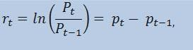
实际上，赫兹量化要预测的不是价格序列本身，而是回报序列。价格变化的对数（不断变化的回报）确定为回报百分比的自然对数：

​

编辑

添加图片注释，不超过 140 字（可选）

其中：

• Pt - 是在时间 t 处的价格序列的值；

• Pt-1 - 是在时间 t-1 处的价格序列的值；

• pt = ln(Pt) - 是自然对数 Pt。

实际上，使用回报要优于使用价格的主要原因是回报具有更好的统计特性。

因此，赫兹量化来创建一个回报指标 ReturnsIndicator.mq5，它对我们非常有用。在这里，我要引用《面向新手的自定义指标》一文，它以易于理解的方式介绍了创建指标的算法。这就是为何在所提及公式已实施的情况下，我只提供代码的原因。我认为这非常简单，无需赘言。

//+------------------------------------------------------------------+ //| Custom indicator iteration function | //+------------------------------------------------------------------+ int OnCalculate(const int rates_total, // size of the array price[] const int prev_calculated, // number of bars available at the previous call const int begin, // index of the array price[] the reliable data starts from const double& price[]) // array for the calculation itself { //--- int start; if(prev_calculated<2) start=1; // start filling ReturnsBuffer[] from the 1-st index, not 0. else start=prev_calculated-1; // set 'start' equal to the last index in the arrays for(int i=start;i<rates_total;i++) { ReturnsBuffer[i]=MathLog(price[i]/price[i-1]); } //--- return value of prev_calculated for next call return(rates_total); } //+------------------------------------------------------------------+

我唯一要强调的是回报序列始终比主序列少 1 个元素。这就是我们从第二个元素开始计算回报数组的原因，第一个元素始终等于 0。

因此，赫兹量化可以使用 ReturnsIndicator 指标获得一个随机时间序列，并将该序列用于研究。

4. 统计检验

现在是时候进行统计检验了。之所以进行统计检验，是为了确定时间序列中是否有任何迹象表明，使用某个模型或其他模型更为合适。在我们的案例中，这个模型就是 GARCH 模型。

使用 Ljung-Box-Pierce Q 检验检查序列的自相关是随机发生还是存在一种关联性。为此，我们需要编写一个新的函数。在这里，自相关指的是同一时间序列 X (t) 在 t1 和 t2 时刻的值之间的相互关系（概率连接）。如果 t1 和 t2 时刻彼此相邻（一个接一个），则我们会寻找序列成员与按某个时间单位偏移的同一序列成员之间的关系：x1, x2, x3, ... и x1+1, x2+1, x3+1, ...移动成员的这种效应称为滞后（时延、延迟）。滞后值可以是任意正数。

现在，我要作补充说明，告诉您以下事项。据我所知，无论是 C++ 还是 MQL5，都没有包含复杂统计计算和平均统计计算的标准程序库。通常，此类计算需要使用专门的统计工具进行。对我而言，使用 Matlab、STATISTICA 9 等工具解决问题要更加容易。然而，我之所以决定不使用外部库，第一是为了展示 MQL5 语言在计算方面具有强大功能，第二是因为我在编写 MQL 代码时学到了不少知识。

现在我们需要进行如下说明。要执行 Q 检验，赫兹量化需要使用复数。这正是我准备复数类的原因。理想情况下，它应该被称为 CComplex。好啦，我让自己放松一下吧。我确信读者已有所准备，不需要我解释什么是复数了。就我个人而言，我不喜欢 MQL5 和 MQL4 中发布的计算傅里叶变换的函数；复数在其中的使用不太明显。此外，还有一个障碍，那就是无法用 MQL5 来覆盖算术运算符。因此我不得不寻求其他方法，并避免使用标准 "C" 标记。我通过以下方式实现复数类：

class Complex { public: double re,im; //re -real component of the complex number, im - imaginary public: void Complex(){}; //default constructor void setComplex(double rE,double iM){re=rE; im=iM;}; //set method (1-st variant) void setComplex(double rE){re=rE; im=0;}; //set method (2-nd variant) void ~Complex(){}; //destructor void opEqual(const Complex &y){re=y.re;im=y.im;}; //operator= void opPlus(const Complex &x,const Complex &y); //operator+ void opPlusEq(const Complex &y); //operator+= void opMinus(const Complex &x,const Complex &y); //operator- void opMult(const Complex &x,const Complex &y); //operator* void opMultEq(const Complex &y); //operator*= (1-st variant) void opMultEq(const double y); //operator*= (2-nd variant) void conjugate(const Complex &y); //conjugation of complex numbers double norm(); //normalization };

例如，两个复数求和的操作可使用 opPlus 方法来进行，减法可使用 opMinus 方法来执行，等等。如果您只是编写代码 c = a + b（其中 a、b、c 是复数），则编译器将显示一个错误。但它将接受以下表达方式：c.opPlus(a,b)。

必要时，用户可扩展复数类的方法集。例如，您可以添加除法运算符。

此外，我也需要用于处理复数数组的辅助函数。这就是我在复数类外部实现此类函数的原因——不是为了在其中循环处理数组元素，而是直接使用由引用传递的数组。共有三个这样的函数：

1. getComplexArr（从一个复数数组返回一个二维实数数组）；

2. setComplexArr（从一个一维实数数组返回一个复数数组）；

3. setComplexArr2（从一个二维实数数组返回一个复数数组）。

应该注意的是，这些函数会返回通过引用传递的数组。这是为什么它们的主体中没有包含 "return" 运算符的原因。不过，根据逻辑推理，尽管其类型为空，我想我们仍可以讨论回报的问题。

复数类和辅助函数在头文件 Complex_class.mqh 中进行了说明。

接下来在执行检验时，赫兹量化将需要自相关函数和傅里叶变换函数。因此，赫兹量化需要一个新类，让我们命名为 CFFT 吧。它将为傅里叶变换处理复数数组。傅里叶类如下所示：

class CFFT { public: Complex Input[]; //input array of complex numbers Complex Output[]; //output array of complex numbers public: bool Forward(const uint N); //direct Fourier transformation bool InverseT(const uint N,const bool Scale=true); //weighted reverse Fourier transformation bool InverseF(const uint N,const bool Scale=false); //non-weighted reverse Fourier transformation void setCFFT(Complex &data1[],Complex &data2[],const uint N); //set method(1-st variant) void setCFFT(Complex &data1[],Complex &data2[]); //set method (2-nd variant) protected: void Rearrange(const uint N); // regrouping void Perform(const uint N,const bool Inverse); // implementation of transformation void Scale(const uint N); // weighting };

应该注意的是，所有傅里叶变换都通过数组执行，数组的长度符合条件 2^N（其中 N 是 2 的幂）。通常来说，数组的长度不等于 2^N。本例中数组的长度增加到 2^N 的值，2^N >= n，其中 n 是数组的长度。添加的数组元素等于 0。这种数组处理是在 autocorr 函数的主体中使用辅助函数 nextpow2 和 pow 函数实现的：

int nFFT=pow(2,nextpow2(ArraySize(res))+1); //power rate of two

因此，如果我们有一个初始数组，其长度 (n) 等于 73585，则函数 nextpow2 将返回值 17，其中 2^17 = 131072。换言之，返回的值比 n 大 pow(2, ceil(log(n)/log(2)))。接下来我们来计算 nFFT 的值：2^(17+1) = 262144. 这将是辅助数组的长度，它从 73585 到 262143 之间的所有元素都等于 0。

傅里叶类在头文件 FFT_class.mqh 中进行了说明。

为节省篇幅，我将跳过有关如何实现 CFFT 类的说明。感兴趣的读者可在随附文件中找到这些说明。现在，赫兹量化来看一下自相关函数。

void autocorr(double &ACF[],double &res[],int nLags) //1-st variant of function /* selective autocorrelation function (ACF) for unidimensional stochastic time series ACF - output array of calculated values of the autocorrelation function; res - array of observation of stochastic time series; nLags - maximum number of lags the ACF is calculated for. */ { Complex Data1[],Data21[], //input arrays of complex numbers Data2[],Data22[], //output arrays of complex numbers cData[]; //array of conjugated complex numbers double rA[][2]; //auxiliary two-dimensional array of real numbers int nFFT=pow(2,nextpow2(ArraySize(res))+1); //power rate of two ArrayResize(rA,nFFT);ArrayResize(Data1,nFFT); //correction of array sizes ArrayResize(Data2,nFFT);ArrayResize(Data21,nFFT); ArrayResize(Data22,nFFT);ArrayResize(cData,nFFT); double rets1[]; //an auxiliary array for observing the series double m=mean(res); //arithmetical mean of the array res ArrayResize(rets1,nFFT); //correction of array size for(int t=0;t<ArraySize(res);t++) //copy the initial array of observation // to the auxiliary one with correction by average rets1[t]=res[t]-m; setComplexArr(Data1,rets1); //set input array of complex numbers CFFT F,F1; //initialize instances of the CFFT class F.setCFFT(Data1,Data2); //initialize data-members for the instance F F.Forward(nFFT); //perform direct Fourier transformation for(int i=0;i<nFFT;i++) { Data21[i].opEqual(F.Output[i]);//assign the values of the F.Output array to the Data21 array; cData[i].conjugate(Data21[i]); //perform conjugation for the array Data21 Data21[i].opMultEq(cData[i]); //multiplication of the complex number by the one adjacent to it //results in a complex number that has only real component not equal to zero } F1.setCFFT(Data21,Data22); //initialize data-members for the instance F1 F1.InverseT(nFFT); //perform weighter reverse Fourier transformation getComplexArr(rA,F1.Output); //get the result in double format after //weighted reverse Fourier transformation for(int i=0;i<nLags+1;i++) { ACF[i]=rA[i][0]; //in the output ACF array save the calculated values //of autocorrelation function ACF[i]=ACF[i]/rA[0][0]; //normalization relatively to the first element } }

因此，赫兹量化已计算了指定滞后值的 ACF 值。现在我们可以将自相关函数用于 Q 检验。检验函数本身会显示如下：

void lbqtest(bool &H[],double &rets[]) /* Function that implements the Q test of Ljung-Box-Pierce H - output array of logic values, that confirm or disprove the zero hypothesis on the specified lag; rets - array of observations of the stochastic time series; */ { double lags[3]={10.0,15.0,20.0}; //specified lags int maxLags=20; //maximum number of lags double ACF[]; ArrayResize(ACF,21); //epmty ACF array double acf[]; ArrayResize(acf,20); //alternate ACF array autocorr(ACF,rets,maxLags); //calculated ACF array for(int i=0;i<20;i++) acf[i]=ACF[i+1]; //remove the first element - one, fill //alternate array double alpha[3]={0.05,0.05,0.05}; //array of levels of significance of the test /*Calculation of array of Q statistics for selected lags according to the formula: L |----| \ Q = T(T+2) || (rho(k)^2/(T-k)), / |----| k=1 where: T is range, L is the number of lags, rho(k) is the value of ACF at the k-th lag. */ double idx[]; ArrayResize(idx,maxLags); //auxiliary array of indexes int len=ArraySize(rets); //length of the array of observations int arrLags[];ArrayResize(arrLags,maxLags); //auxiliary array of lags double stat[]; ArrayResize(stat,maxLags); //array of Q statistics double sum[]; ArrayResize(sum,maxLags); //auxiliary array po sums double iACF[];ArrayResize(iACF,maxLags); //auxiliary ACF array for(int i=0;i<maxLags;i++) { //fill: arrLags[i]=i+1; //auxiliary array of lags idx[i]=len-arrLags[i]; //auxiliary array of indexes iACF[i]=pow(acf[i],2)/idx[i]; //auxiliary ACF array } cumsum(sum,iACF); //sum the auxiliary ACF array //by progressive total for(int i=0;i<maxLags;i++) stat[i]=sum[i]*len*(len+2); //fill the array Q statistics double stat1[]; //alternate of the array of Q statistics ArrayResize(stat1,ArraySize(lags)); for(int i=0;i<ArraySize(lags);i++) stat1[i]=stat[lags[i]-1]; //fill the alternate array of specified lags double pValue[ArraySize(lags)]; //array of 'p' values for(int i=0;i<ArraySize(lags);i++) { pValue[i]=1-gammp(lags[i]/2,stat1[i]/2); //calculation of 'p' values H[i]=alpha[i]>=pValue[i]; //estimation of zero hypothesis } }

于是，赫兹量化的函数执行 Ljung-Box-Pierce Q 检验并返回指定滞后值的逻辑值数组。赫兹量化需要指出，Ljung-Box 检验就是所谓的便利的检定（综合检验）。它意味着将不超过指定滞后值的一些滞后值组用于检查自相关的存在。通常而言，自相关的检查可包含第 10 个、第 15 个和第 20 个便利的滞后值。基于 H 数组元素的最后的值（即从第 1 个到第 20 个滞后值）得出了整个序列中是否存在自相关的结论。

如果数组中的元素等于 false，则表示接受之前滞后值和选定滞后值无自相关这一零假设。换言之，当值为 false 时，则表示不存在自相关。否则，检验会证明存在自相关。因此，当值为 true 时，零假设以外的假设将会被接受。

有时候，也会发生在回报序列中未找到自相关的情况。在这种情况下，为了提高精确度，可检验回报的平方。检验初始回报序列时，也会以同样的方式做出接受或拒绝零假设的最终决定。为什么要使用回报平方？- 通过这种方式，赫兹量化人为增加了分析序列可能具有的非随机自相关要素，然后在受信限值的初始值的范围内对其进一步确定。理论上来说，您可以使用回报的平方或其他次幂。但这是不必要的统计负载，导致检验没有意义。

在 Q 检验函数主体的末尾，当计算了 "p" 值后，函数 gammp(x1/2,x2/2) 就会出现。它可以针对相应元素进行不完整的 gamma 函数计算。实际上，我们需要一个 χ2 分布（卡方分布）的累积函数。但它是 Gamma 分布的一个特例。

一般而言，要证明使用 GARCH 模型是否合适，只需获得 Q 检验任何滞后值的一个正值即可。此外，计量经济学家也进行了其他检验 - Engle 的 ARCH 检验，用于检查是否存在传统的异方差性。然而对于时间序列而言，我认为 Q 检验已经足够。它是最普遍的检验。

现在我们已有了进行检验所需的所有函数，需要考虑在屏幕上显示所获得的结果了。为此，我编写了另一个函数 lbqtestInfo，它将以消息窗口的形式显示计量经济学结果，并在分析的交易品种的图表上显示自相关图。

让我们通过一个示例来看下结果。我选择 USDJPY 作为分析的首个交易品种。首先，我打开该交易品种的线形图（取收盘价）并加载自定义指标 ReturnsIndicator 以说明回报序列。图表应尽可能地简化，以更好地显示指标的波动集群性。接下来我会执行脚本 GarchTest。或许您的屏幕分辨率与我的不同，脚本会询问您图解所需的像素大小。我这边的标准是 700*250。