


线性预测编码(Linear Predictive Coding, LPC)技术在数字信号处理教材里面可以看到,并不是语音信号处理才会涉及到的基础技术。这篇文章主要是回顾一下LPC的基础内容,因为在语音信号处理的相关研究方法中,基于LPC的语音信号处理技术表现出了优异的性能,尤其是针对语音去混响研究[1,2,3]。
语音是由我们的发声系统产生,该系统可以由简单的声源和声道模型来进行模拟。声源是由声带产生的,声带向声道提供激励信号,这种激励可以是周期性的或非周期性的。当声带处于发声状态(振动)时,会产生有声声音(例如,元音);而当声带处于无声状态时,会产生无声声音(例如,辅音)。声道可以看作是一个滤波器,它可以对来自声带的激励信号频谱进行整形以产生各种声音。
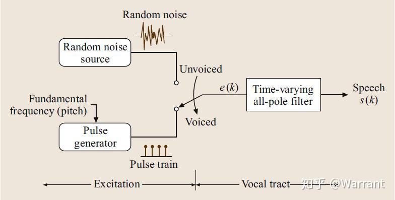
图1 语音生成模型
图1提供了一个实用化的语音生成工程模型,LPC正是基于这个模型的语音生成技术。在该模型中,语音信号是由一个激励信号  经过一个时变的全极点滤波器产生。全极点滤波器的系数取决于所产生的特定声音的声道形状。激励信号
 要么是浊音语音的脉冲序列,要么是无声声音的随机噪声。生成语音信号
  可以表示为
可以表示为

其中,  是滤波器的阶数,
  是滤波器的系数。LPC就是在已知 的情况下获取 .
求取 最常用的一个方法就是最小化真实信号与预测信号之间的均方误差(Mean Squared Error, MSE)。MSE函数可以表示为
![~~~~~~~~~~~~~~~~~~~~~~~~~ \begin{equation}\label{wpeeq3} J=E\left[e^{2}(k)\right]=E\left[\left(s(k)-\sum_{p=1}^{P}a_{p}s(k-p)\right)^{2}\right], ~~~~~~~~~~~~~(2) \end{equation}](https://i-blog.csdnimg.cn/blog_migrate/9383d7bef46cdbf09ff337333cb2f8c4.png)
然后,计算  关于每个滤波器系数的偏导,并令其值等于0,可得

通过对(3)计算,可以得到
![~~~~~~~~~~~~~~~~~~ \begin{equation}\label{wpeeq5} \sum_{u=1}^{P}a_{u}E\left[s(k-p)s(k-u)\right]=E\left[s(k)s(k-u)\right],~1\leq u\leq p, ~~~~(4) \end{equation}](https://i-blog.csdnimg.cn/blog_migrate/f7687afa0d19f527a0bae8ed5c16a781.png)
其中,  。用数值
。用数值  分别替换(4)中的变量
  ,我们可以得到 个关于滤波器系数的线性方程组,求解该线性方程组,即可得到滤波器系数的解。求解该方程组最常用高效的方法是
  算法。
算法。
Introduction to CELP Coding
Speex is based on CELP, which stands for Code Excited Linear Prediction. This section attempts to introduce the principles behind CELP, so if you are already familiar with CELP, you can safely skip to section. The CELP technique is based on three ideas:
- The use of a linear prediction (LP) model to model the vocal tract
- The use of (adaptive and fixed) codebook entries as input (excitation) of the LP model
- The search performed in closed-loop in a ``perceptually weighted domain''
This section describes the basic ideas behind CELP. This is still a work in progress.
Source-Filter Model of Speech Prediction
The source-filter model of speech production assumes that the vocal cords are the source of spectrally flat sound (the excitation signal), and that the vocal tract acts as a filter to spectrally shape the various sounds of speech. While still an approximation, the model is widely used in speech coding because of its simplicity.Its use is also the reason why most speech codecs (Speex included) perform badly on music signals. The different phonemes can be distinguished by their excitation (source) and spectral shape (filter). Voiced sounds (e.g. vowels) have an excitation signal that is periodic and that can be approximated by an impulse train in the time domain or by regularly-spaced harmonics in the frequency domain. On the other hand, fricatives (such as the "s", "sh" and "f" sounds) have an excitation signal that is similar to white Gaussian noise. So called voice fricatives (such as "z" and "v") have excitation signal composed of an harmonic part and a noisy part.
The source-filter model is usually tied with the use of Linear prediction. The CELP model is based on source-filter model, as can be seen from the CELP decoder illustrated in Figure 1.
|
|
![\includegraphics[width=0.45\paperwidth,keepaspectratio]{celp_decoder}](https://www.speex.org/docs/manual/speex-manual/img7.png)
Linear Prediction (LPC)
Linear prediction is at the base of many speech coding techniques, including CELP. The idea behind it is to predict the signal ![]() using a linear combination of its past samples:
using a linear combination of its past samples:
![$\displaystyle y[n]=\sum_{i=1}^{N}a_{i}x[n-i]$](https://www.speex.org/docs/manual/speex-manual/img9.png)
where ![]() is the linear prediction of
is the linear prediction of ![]() . The prediction error is thus given by:
. The prediction error is thus given by:
![$\displaystyle e[n]=x[n]-y[n]=x[n]-\sum_{i=1}^{N}a_{i}x[n-i]$](https://www.speex.org/docs/manual/speex-manual/img11.png)
The goal of the LPC analysis is to find the best prediction coefficients ![]() which minimize the quadratic error function:
which minimize the quadratic error function:
![$\displaystyle E=\sum_{n=0}^{L-1}\left[e[n]\right]^{2}=\sum_{n=0}^{L-1}\left[x[n]-\sum_{i=1}^{N}a_{i}x[n-i]\right]^{2}$](https://www.speex.org/docs/manual/speex-manual/img13.png)
That can be done by making all derivatives ![]() equal to zero:
equal to zero:
![$\displaystyle \frac{\partial E}{\partial a_{i}}=\frac{\partial}{\partial a_{i}}\sum_{n=0}^{L-1}\left[x[n]-\sum_{i=1}^{N}a_{i}x[n-i]\right]^{2}=0$](https://www.speex.org/docs/manual/speex-manual/img15.png)
For an order ![]() filter, the filter coefficients
filter, the filter coefficients ![]() are found by solving the system
are found by solving the system ![]() linear system
linear system ![]() , where
, where
![$\displaystyle \mathbf{R}=\left[\begin{array}{cccc} R(0) & R(1) & \cdots & R(N-1... ...& \vdots & \ddots & \vdots\\ R(N-1) & R(N-2) & \cdots & R(0)\end{array}\right]$](https://www.speex.org/docs/manual/speex-manual/img18.png)
![$\displaystyle \mathbf{r}=\left[\begin{array}{c} R(1)\\ R(2)\\ \vdots\\ R(N)\end{array}\right]$](https://www.speex.org/docs/manual/speex-manual/img19.png)
with ![]() , the auto-correlation of the signal
, the auto-correlation of the signal ![]() , computed as:
, computed as:
![$\displaystyle R(m)=\sum_{i=0}^{N-1}x[i]x[i-m]$](https://www.speex.org/docs/manual/speex-manual/img21.png)
Because ![]() is toeplitz hermitian, the Levinson-Durbin algorithm can be used, making the solution to the problem
is toeplitz hermitian, the Levinson-Durbin algorithm can be used, making the solution to the problem ![]() instead of
instead of ![]() . Also, it can be proven that all the roots of
. Also, it can be proven that all the roots of ![]() are within the unit circle, which means that
are within the unit circle, which means that ![]() is always stable. This is in theory; in practice because of finite precision, there are two commonly used techniques to make sure we have a stable filter. First, we multiply
is always stable. This is in theory; in practice because of finite precision, there are two commonly used techniques to make sure we have a stable filter. First, we multiply ![]() by a number slightly above one (such as 1.0001), which is equivalent to adding noise to the signal. Also, we can apply a window to the auto-correlation, which is equivalent to filtering in the frequency domain, reducing sharp resonances.
by a number slightly above one (such as 1.0001), which is equivalent to adding noise to the signal. Also, we can apply a window to the auto-correlation, which is equivalent to filtering in the frequency domain, reducing sharp resonances.
Pitch Prediction
During voiced segments, the speech signal is periodic, so it is possible to take advantage of that property by approximating the excitation signal ![]() by a gain times the past of the excitation:
by a gain times the past of the excitation:
![]()
where ![]() is the pitch period,
is the pitch period, ![]() is the pitch gain. We call that long-term prediction since the excitation is predicted from
is the pitch gain. We call that long-term prediction since the excitation is predicted from ![]() with
with ![]() .
.
Innovation Codebook
The final excitation ![]() will be the sum of the pitch prediction and an innovation signal
will be the sum of the pitch prediction and an innovation signal ![]() taken from a fixed codebook, hence the name Code Excited Linear Prediction. The final excitation is given by:
taken from a fixed codebook, hence the name Code Excited Linear Prediction. The final excitation is given by:
![]()
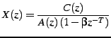
The quantization of ![]() is where most of the bits in a CELP codec are allocated. It represents the information that couldn't be obtained either from linear prediction or pitch prediction. In the z-domain we can represent the final signal
is where most of the bits in a CELP codec are allocated. It represents the information that couldn't be obtained either from linear prediction or pitch prediction. In the z-domain we can represent the final signal ![]() as
as
Noise Weighting
Most (if not all) modern audio codecs attempt to ``shape'' the noise so that it appears mostly in the frequency regions where the ear cannot detect it. For example, the ear is more tolerant to noise in parts of the spectrum that are louder and vice versa. In order to maximize speech quality, CELP codecs minimize the mean square of the error (noise) in the perceptually weighted domain. This means that a perceptual noise weighting filter ![]() is applied to the error signal in the encoder. In most CELP codecs,
is applied to the error signal in the encoder. In most CELP codecs, ![]() is a pole-zero weighting filter derived from the linear prediction coefficients (LPC), generally using bandwidth expansion. Let the spectral envelope be represented by the synthesis filter
is a pole-zero weighting filter derived from the linear prediction coefficients (LPC), generally using bandwidth expansion. Let the spectral envelope be represented by the synthesis filter ![]() , CELP codecs typically derive the noise weighting filter as:
, CELP codecs typically derive the noise weighting filter as:
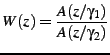 | (1) |
where ![]() and
and ![]() in the Speex reference implementation. If a filter
in the Speex reference implementation. If a filter ![]() has (complex) poles at
has (complex) poles at ![]() in the
in the ![]() -plane, the filter
-plane, the filter ![]() will have its poles at
will have its poles at ![]() , making it a flatter version of
, making it a flatter version of ![]() .
.
The weighting filter is applied to the error signal used to optimize the codebook search through analysis-by-synthesis (AbS). This results in a spectral shape of the noise that tends towards ![]() . While the simplicity of the model has been an important reason for the success of CELP, it remains that
. While the simplicity of the model has been an important reason for the success of CELP, it remains that ![]() is a very rough approximation for the perceptually optimal noise weighting function. Fig. 2 illustrates the noise shaping that results from Eq. 1. Throughout this paper, we refer to
is a very rough approximation for the perceptually optimal noise weighting function. Fig. 2 illustrates the noise shaping that results from Eq. 1. Throughout this paper, we refer to ![]() as the noise weighting filter and to
as the noise weighting filter and to ![]() as the noise shaping filter (or curve).
as the noise shaping filter (or curve).
|
|
![\includegraphics[width=0.45\paperwidth,keepaspectratio]{ref_shaping}](https://www.speex.org/docs/manual/speex-manual/img47.png)
Analysis-by-Synthesis
One of the main principles behind CELP is called Analysis-by-Synthesis (AbS), meaning that the encoding (analysis) is performed by perceptually optimising the decoded (synthesis) signal in a closed loop. In theory, the best CELP stream would be produced by trying all possible bit combinations and selecting the one that produces the best-sounding decoded signal. This is obviously not possible in practice for two reasons: the required complexity is beyond any currently available hardware and the ``best sounding'' selection criterion implies a human listener.
In order to achieve real-time encoding using limited computing resources, the CELP optimisation is broken down into smaller, more manageable, sequential searches using the perceptual weighting function described earlier.
参考文献
[1]Yoshioka T, Nakatani T, Miyoshi M. An integrated method for blind separation and dereverberation of convolutive audio mixtures[C]// Signal Processing Conference, 2008, European. IEEE, 2008:1-5.
[2]Nakatani T, Yoshioka T, Kinoshita K, et al. Blind speech dereverberation with multi-channel linear prediction based on short time fourier transform representation[C]// IEEE International Conference on Acoustics, Speech and Signal Processing. IEEE, 2008:85-88.
[3]Nakatani T, Yoshioka T, Kinoshita K, et al. Speech Dereverberation Based on Variance-Normalized Delayed Linear Prediction[J]. IEEE Transactions on Audio Speech & Language Processing, 2010, 18(7):1717-1731.


 810
810

 被折叠的 条评论
为什么被折叠?
被折叠的 条评论
为什么被折叠?
 到【灌水乐园】发言


