NSGA2多目标优化算法的MATLAB仿真

目录

1.算法描述

2.仿真效果预览

3.MATLAB核心程序

4.完整MATLAB

---

1.算法描述

       首先将一群具有多个目标的个体（解集，或者说线代里的向量形式）作为父代初始种群，在每一次迭代中，GA操作后合并父代于自带。通过非支配排序，我们将所有个体分不到不同的pareto最优前沿层次。然后根据不同层次的顺序从pareto最优前沿选择个体作为下一个种群。出于遗传算法中的“物种多样性”保护，还计算量“拥挤距离”。拥挤距离比较将算法各阶段的选择过程引向一致的前沿。    

       与单目标（遗传算法）最大的不同就是进行选择操作之前进行快速非支配排序，这一步也是为了选择操作而来的，选择哪些、怎么选是通过非快速支配排序来的。这就不像单目标，挑好的选就行了。
       支配： 在多目标优化问题中，如果个体p至少有一个目标比个体q好，而且个体p中的所有目标都不比个体q差，那么称个体p支配个体q。

      序值： 如果p支配q，那么p的序值比q低。如果p和q互不支配，那么p和q有相同的序值。

      拥挤距离：用来计算某前端中的某个体与该前端中其他个体之间的距离，用以表征个体间的拥挤程度。希望pareto解出来之后，点与点之间距离是相近的，不要太多的聚集在某个地方。用某个点与前后两个点之间的xy的距离和表示。算法会选择拥挤距离大的去领头。

     快速非支配排序：快速非支配排序就是将解集分解为不同次序的Pareto前沿的过程。将一组解分成n个集合：rank1,rank2…rankn,每个集合中所有的解都互不支配，但ranki中的任意解支配rankj中的任意解（i<j）.

综上所述，NSGAII的步骤如下所示：

步骤1：编码。遗传算法在进行搜索之前，将变量编成一个定长的编码——用二进制字符串来表示，这些字符串的不同组合，
便构成了搜索空间不同的搜索点。
步骤2：产生初始群体。随机产生N个字符串，每个字符串代表一个个体。
步骤3：按目标函数的个数分割子群体，对每个子群体进行如下操作：
1)计算目标函数值(此步调用ANSYs有限元程序，将ANSYS有限元程序得到的后处理结果传给MATLAB程序作为目标函数值)；
2)计算每个个体的适应度，本文中采用线性排序法和选择压差为2估算适应度；
3)用随机遍历抽样方法在每个子种群中选择个体。
步骤4：将每个子种群中选择出的个体进行合并。
步骤5：交叉操作。本文中采用的是单点交叉操作。
步骤6：变异。对个体按给定的概率进行变异，形成新一代群体。
步骤7：将步骤6产生的个体合重复进行步骤3～ 步骤6的操作，直至完成规定的遗传迭代总次数。

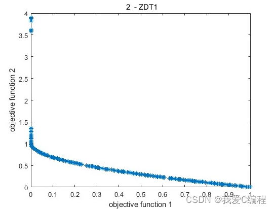
2.仿真效果预览

matlab2022a仿真结果如下：

3.MATLAB核心程序

 
%% Description
%pop_size 染色体的数目
%gen_max  最大遗传代数
%gen_count 目前的迭代数
%M 目标函数的数量
%no_runs 运行次数
%xl,xu为设计变量的下限和上限
%最终的Pareto解在变量’parto_rank1’中，设计变量在coumns(1:V),目标函数在（V+1，V+M）
%约束在（V+M+1),排序在（V+M+2),拥挤距离在（V+M+3)中
 
%% code starts
M=2;
p=2;
pop_size=200;           % Population size
no_runs=1;              % Number of runs
gen_max=500;            % MAx number of generations - stopping criteria
fname='test_case';      % Objective function and constraint evaluation
 
if p==13,  % OSY
    pop_size=100; 
    no_runs=10;
end;                   
if (p==2 | p==5 | p==7), gen_max=1000; end;
 
if p<=9     % Unconstrained test functions
tV=[2;30;3;1;30;4;30;10;10];
V=tV(p);
txl=[-5*ones(1,V);zeros(1,V);-5*ones(1,V);-1000*ones(1,V);zeros(1,V);-1/sqrt(V)*ones(1,V);zeros(1,V); 0 -5*ones(1,V-1);zeros(1,V)]; 
txu=[10*ones(1,V); ones(1,V);5*ones(1,V);1000*ones(1,V);ones(1,V);1/sqrt(V) *ones(1,V);ones(1,V);1 5*ones(1,V-1);ones(1,V)];
xl=(txl(p,1:V));            % lower bound vector
xu=(txu(p,1:V));            % upper bound vectorfor 
etac = 20;                  % distribution index for crossover
etam = 20;                  % distribution index for mutation / mutation constant
else         % Constrained test functions
p1=p-9;
tV=[2;2;2;6;2];
V=tV(p1);
txl=[0 0 0 0 0 0;-20 -20 0 0 0 0;0 0 0 0 0 0;0 0 1 0 1 0;0.1 0 0 0 0 0]; 
txu=[5 3 0 0 0 0;20 20 0 0 0 0;pi pi 0 0 0 0;10 10 5 6 5 10;1 5 0 0 0 0];
xl=(txl(p1,1:V));           % lower bound vector
xu=(txu(p1,1:V));           % upper bound vectorfor i=1:NN
etac = 20;                  % distribution index for crossover
etam = 100;                 % distribution index for mutation / mutation constant
end
pm=1/V;                     % Mutation Probability
 
Q=[];
for run = 1:no_runs
    
%% Initial population 
xl_temp=repmat(xl, pop_size,1);
xu_temp=repmat(xu, pop_size,1);
x = xl_temp+((xu_temp-xl_temp).*rand(pop_size,V));
%% Evaluate objective function
for i =1:pop_size
[ff(i,:) err(i,:)] =feval(fname, x(i,:));           % Objective function evaulation 
end
error_norm=normalisation(err);                      % Normalisation of the constraint violation
population_init=[x ff error_norm];
[population front]=NDS_CD_cons(population_init);    % Non domination Sorting on initial population
    
%% Generation Starts
for gen_count=1:gen_max
% selection (Parent Pt of 'N' pop size)
parent_selected=tour_selection(population);                     % 10 Tournament selection
%% Reproduction (Offspring Qt of 'N' pop size)
child_offspring  = genetic_operator(parent_selected(:,1:V));    % SBX crossover and polynomial mutation
 
for ii = 1:pop_size
[fff(ii,:) err(ii,:)]=feval(fname, child_offspring(ii,:));      % objective function evaluation for offspring
end
 
error_norm=normalisation(err);                                  
child_offspring=[child_offspring fff error_norm];
 
%% INtermediate population (Rt= Pt U Qt of 2N size)
population_inter=[population(:,1:V+M+1) ; child_offspring(:,1:V+M+1)];
[population_inter_sorted front]=NDS_CD_cons(population_inter);              % Non domination Sorting on offspring
%% Replacement - N
new_pop=replacement(population_inter_sorted, front);
population=new_pop;
end
new_pop=sortrows(new_pop,V+1);
paretoset(run).trial=new_pop(:,1:V+M+1);
Q = [Q; paretoset(run).trial];                      % Combining Pareto solutions obtained in each run
end
 
%% Result and Pareto plot
if run==1
plot(new_pop(:,V+1),new_pop(:,V+2),'*')
else                                        
[pareto_filter front]=NDS_CD_cons(Q);               % Applying non domination sorting on the combined Pareto solution set
rank1_index=find(pareto_filter(:,V+M+2)==1);        % Filtering the best solutions of rank 1 Pareto
pareto_rank1=pareto_filter(rank1_index,1:V+M)
plot(pareto_rank1(:,V+1),pareto_rank1(:,V+2),'*')   % Final Pareto plot
A127

4.完整MATLAB

V