机器学习之逻辑回归 Logistic Regression（二）Python实现

参考 http://blog.csdn.net/han_xiaoyang/article/details/49123419

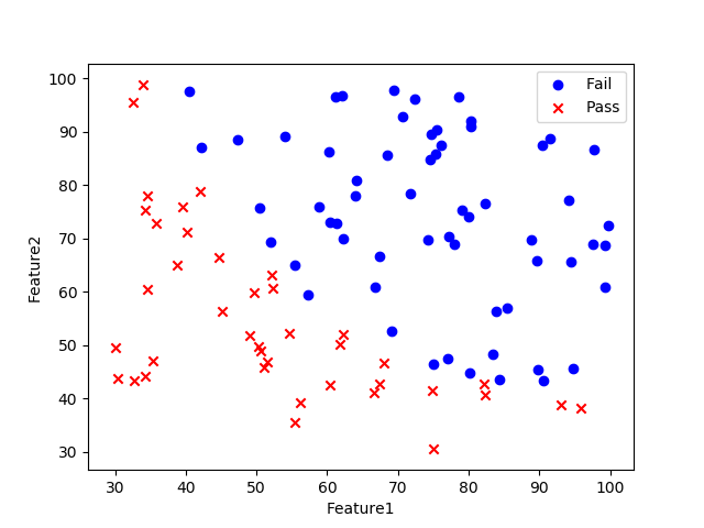
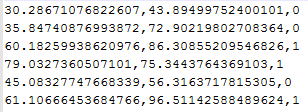
        在一组数据上做逻辑回归，数据格式如下：

         先来看数据分布，代码如下：

from numpy import loadtxt, where
from pylab import scatter, show, legend, xlabel, ylabel

data = loadtxt("data1.txt", delimiter=',')
X = data[:, 0:2]
y = data[:, 2]
pos = where(y==1)
neg = where(y==0)
scatter(X[pos, 0], X[pos, 1], marker='o', c='b')
scatter(X[neg, 0], X[neg, 1], marker='x', c='r')
xlabel("Feature1")
ylabel("Feature2")
legend(["Fail", "Pass"])
show()

import matplotlib.pyplot as plt
import numpy as np

def loadData():
	data = loadtxt("data1.txt", delimiter=',')
	m,n = shape(data)
	train_x = data[:, 0:2]
	train_y = data[:, 2]
	X1 = np.ones((m,1))
	train_x = np.concatenate((X1, train_x), axis = 1)
	return(mat(train_x), mat(train_y).transpose())

def sigmoid(z):
	''' Compute sigmoid function '''
	gz = 1.0/(1.0+exp(-z))
	return(gz)

def trainLogRegress(train_x, train_y):
	''' Compute cost given predicted and actual values '''
	m = train_x.shape[0]  # number of training examples
	weight = zeros((3,1))
	alpha = 0.001
	maxCycles = 9999
	for k in range(maxCycles):
		h = sigmoid(train_x * weight)
		error = train_y - h
		weight = weight + alpha * train_x.transpose() * error 
		print(weight)
		#J = -1.0/m*(yMat.T*log(h)+(1-yMat.T)*log(1-h))
	return weight

def testLogRegress(weight, test_x, test_y):
	m = test_x.shape[0]
	match = 0
	for i in range(m):
		predict = sigmoid(test_x[i, :] * weight)[0,0] > 0.5
		if predict == bool(test_y[i,0]):
			match += 1
	return float(match) / m
		
def showLogRegress(weight, train_x, train_y):
	m = train_x.shape[0]
	# draw all samples
	for i in range(m):
		if int(train_y[i, 0]) == 0:
			plt.plot(train_x[i, 1], train_x[i, 2], 'xr')
		elif int(train_y[i, 0]) == 1:
			plt.plot(train_x[i, 1], train_x[i, 2], 'ob')
	# draw the classify line
	min_x = min(train_x[:, 1])[0, 0]
	max_x = max(train_x[:, 1])[0, 0]
	y_min_x = float(-weight[0,0] - weight[1,0] * min_x) / weight[2,0]
	y_max_x = float(-weight[0,0] - weight[1,0] * max_x) / weight[2,0]
	print(min_x, max_x, y_min_x, y_max_x)
	plt.plot([min_x, max_x], [y_min_x, y_max_x], '-g')
	plt.xlabel("Feature1")
	plt.ylabel("Feature2")
	plt.show()
	
train_x, train_y = loadData()
weight = trainLogRegress(train_x, train_y)
accuracy = testLogRegress(weight, train_x, train_y)
print(accuracy)
showLogRegress(weight, train_x, train_y)

总结
       最后总结一下逻辑回归。它始于输出结果为有实际意义的连续值的线性回归，但是线性回归对于分类的问题没有办法准确而又具备鲁棒性地分割，因此设计出了逻辑回归这样一个算法，它的输出结果表征了某个样本属于某类别的概率。
       逻辑回归的成功之处在于，将原本输出结果范围可以非常大的θTX 通过sigmoid函数映射到(0,1)，从而完成概率的估测。
        而直观地在二维空间理解逻辑回归，是sigmoid函数的特性，使得判定的阈值能够映射为平面的一条判定边界，当然随着特征的复杂化，判定边界可能是多种多样的样貌，但是它能够较好地把两类样本点分隔开，解决分类问题。
       求解逻辑回归参数的传统方法是梯度下降，构造为凸函数的代价函数后，每次沿着偏导方向(下降速度最快方向)迈进一小部分，直至N次迭代后到达最低点。