


调试设置
-
Debug 设置
{
    // 使用 IntelliSense 了解相关属性。
    // 悬停以查看现有属性的描述。
    // 欲了解更多信息,请访问: https://go.microsoft.com/fwlink/?linkid=830387
    "version": "0.2.0",
    "configurations": [
            {
	            "name": "Python: Current File",
	            "type": "python",
	            "request": "launch",
	            "program": "val.py",
	            "console": "integratedTerminal",
	            "justMyCode": true,
	            "args":["--data", "coco128.yaml",
                    	"--workers", "0",
                    	"--batch-size", "1"]
        	}
         ]
}
其它参数则是使用默认,其中 【–workers=0】表示仅仅使用主线程读取数据。那么调试过程中,每次读取的数据是同一个数据,便于打印关键变量的变化。
-
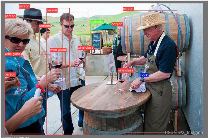
调试数据
使用的是【coco.yaml】数据, 图片【000000000308.jpg】,总共有4类,13个目标框,如下图所示,
前置知识
理解mAP的计算过程,有一些基本的概念和专业术语需要弄清楚。参考博客链接:指标评估 —— AP & mAP 详细解读.
整体结构
指标评估主要涉及两个脚本文件,【val.py】:指标评估的主要流程控制;【metrics.py】:核心功能的具体代码实现,比如AP,mAP的计算过程,PR曲线的绘制等。
-
脚本【val.py】的大致结构如下,
def save_one_txt(predn, save_conf, shape, file): # save txt def save_one_json(predn, jdict, path, class_map): # Save one JSON result {"image_id": 42, # "category_id": 18, # "bbox": [258.15, 41.29, 348.26, 243.78], # "score": 0.236} def process_batch(detections, labels, iouv): """ Return correct predictions matrix. Both sets of boxes are in (x1, y1, x2, y2) format. Arguments: detections (Array[N, 6]), x1, y1, x2, y2, conf, class labels (Array[M, 5]), class, x1, y1, x2, y2 Returns: correct (Array[N, 10]), for 10 IoU levels """ # 计算指标的关键函数之一 # iou:[0.5:0.95],10个不同的iou阈值下,计算标签与预测的匹配结果,存于矩阵,标记是否预测正确 @torch.no_grad() def run( data, weights=None, # model.pt path(s) batch_size=32, # batch size imgsz=640, # inference size (pixels) conf_thres=0.001, # confidence threshold iou_thres=0.6, # NMS IoU threshold task='val', # train, val, test, speed or study device='', # cuda device, i.e. 0 or 0,1,2,3 or cpu workers=8, # max dataloader workers (per RANK in DDP mode) ... ... ): """ # 函数run()的处理流程如下: 1. 加载模型; 2. 加载数据; 3. 网络预测,NMS处理; 4. 计算AP,mAP; 5. 绘制指标图; 6. 保存结果; """ def parse_opt(): # 运行相关参数定义 def main(opt): # 入口函数 run(**vars(opt)) if __name__ == "__main__": opt = parse_opt() main(opt) -
脚本【metric.py】的大致结构如下,
包含核心的功能实现代码def ap_per_class(tp, conf, pred_cls, target_cls, plot=False, save_dir='.', names=(), eps=1e-16): """ Compute the average precision, given the recall and precision curves. Source: https://github.com/rafaelpadilla/Object-Detection-Metrics. # Arguments tp: True positives (nparray, nx1 or nx10). conf: Objectness value from 0-1 (nparray). pred_cls: Predicted object classes (nparray). target_cls: True object classes (nparray). plot: Plot precision-recall curve at mAP@0.5 save_dir: Plot save directory # Returns The average precision as computed in py-faster-rcnn. """ # 计算AP,F1,Presion,Recall,绘制指标图 def compute_ap(recall, precision): """ Compute the average precision, given the recall and precision curves # Arguments recall: The recall curve (list) precision: The precision curve (list) # Returns Average precision, precision curve, recall curve """ # 根据PR曲线,计算每一类的AP值 # 两种方法:插值101点或者连续点计算曲线下方的面积 class ConfusionMatrix: # Updated version of https://github.com/kaanakan/object_detection_confusion_matrix def __init__(self, nc, conf=0.25, iou_thres=0.45): self.matrix = np.zeros((nc + 1, nc + 1)) self.nc = nc # number of classes self.conf = conf self.iou_thres = iou_thres # 计算混淆矩阵 def bbox_iou(box1, box2, xywh=True, GIoU=False, DIoU=False, CIoU=False, eps=1e-7): # Returns Intersection over Union (IoU) of box1(1,4) to box2(n,4) def plot_pr_curve(px, py, ap, save_dir=Path('pr_curve.png'), names=()): # 绘制PR曲线
核心函数
-
process_batch
函数作用:为计算AP,mAP作准备。
基本思想:在一组不同的IOU阈值下,标记每一个预测框是正确预测,还是错误预测,正确标记为True,错误标记为False,标记结果存于【correct】矩阵。经过NMS处理后,存在预测框和标签框不是一一对应的关系,为了后续计算mAP,需要保证一个标签框对应一个预测框。
去除重复框:当一个预测框对应多个标签框时,需要根据iou值的大小,最大iou值的框标记为正确预测,其它iou值的重复预测框均为错误预测;当一个标签框对应多个预测框时,根据置信度分数筛选,置信度最大的预测框为正确预测,其它置信度分数的则为错误预测。该函数的基本流程如下:
(1)初始化返回矩阵 correct,shape=[num_predicts,10],num_predicts:网络预测的框经过NMS处理后剩下的数量;10:10个不同的iou阈值;
(2)计算所有预测框和真实框两两之间的交并比值,形状[num_gt, num_predicts];
(3)标记正确预测的类别,存于correct_class,形状[num_gt, num_predicts];
(4)循环每一个iou阈值,并计算该iou值下的正确预测的框,循环处理流程为(5)-(9);
(5)筛选出类别预测正确,并且iou大于阈值的框,返回索引,存于x;
(6)x不为空的情况下,将标签框的id,预测框的id,以及对应的iou值组合为新的矩阵,存于matches;
(7)对IOU进行从大到小进行排序,进而对matches进行排序;
(8)去除重复的预测框和真实框,保证预测框和预测框一一对应;
(9)将新的matches[:,1]取出,更新correct相应位置为True;
返回Tensor的解释:
correct:[num_detections, 10],正确预测框被标记为True;每一列对应不同的iou阈值下,预测框的正确与否;每一行标记类别预测正确,且iou最大的框的id为true,其它为false;
一些问题,思考:
(1)为何要根据iou对 matches进行排序?保留最大的iou预测框。
(2)为何要去除matches中重复的预测框和真实框?一个真实框只能有一个正确的预测框。def process_batch(detections, labels, iouv): """ Return correct predictions matrix. Both sets of boxes are in (x1, y1, x2, y2) format. Arguments: detections (Array[N, 6]), x1, y1, x2, y2, conf, class labels (Array[M, 5]), class, x1, y1, x2, y2 Returns: correct (Array[N, 10]), for 10 IoU levels """ # detections:[300,6],iouv:[10]=[0.5,0.55,0.60,0.65,0.70,0.75,0.80,0.85,0.90,0.95] # labels: [13,5] # correct: [300,10],每一列表示一个iou阈值下,该检测框是否为正样本; # 300:表示预测框经过NMS处理后剩下的数量,10:iou阈值的数量 # 是:true;否:false correct = np.zeros((detections.shape[0], iouv.shape[0])).astype(bool) # 两两计算预测框和真实框的IOU值, 得到iou: [13,300] # 矩阵的每一个位置:记录每一个标签框与预测框的IOU值 iou = box_iou(labels[:, 1:], detections[:, :4]) # 标记正确预测的类别,correct_class=[13,300] # 该矩阵的每一个位置:记录预测框是否与标签框的类别一致 correct_class = labels[:, 0:1] == detections[:, 5] # iouv: [0.5:0.05:0.95],计算每一个iou下的正确预测的情况 for i in range(len(iouv)): # x: i=0, len(x)=2, # x[0]:true的行索引,len(x[0])=26,表示有26个位置iou既大于阈值,且类别预测正确 # x[1]:true的列索引, x = torch.where((iou >= iouv[i]) & correct_class) # IoU > threshold and classes match if x[0].shape[0]: # matches: [26,3],存储当前iou阈值下,预测的情况 # matches[:,0]: 标签框的id索引 # matches[:,1]: 预测框的id索引 # matches[:,2]: iou的具体值 matches = torch.cat((torch.stack(x, 1), iou[x[0], x[1]][:, None]), 1).cpu().numpy() # [label, detect, iou] if x[0].shape[0] > 1: # 根据iou值对matches进行从大到小排序 matches = matches[matches[:, 2].argsort()[::-1]] # 含义:每一个预测框只能出现一次,如果一个预测框(表现为matches[:, 1]相同的数值)与多个gt的iou大于阈值,则保留iou最大的一个 # 去除重复的检测框id,保留重复id中最大iou的id,留下一个最大的iou框 matches = matches[np.unique(matches[:, 1], return_index=True)[1]] # matches = matches[matches[:, 2].argsort()[::-1]] # 含义:一个gt不能对应多个预测框;此时的matche[:,1]已经从小到大进行排序(在NMS阶段,得分高的id小), # 此时按照matches[:,0]进行排序的过程中,会去除重复的标签id;实际上,结合已经排序的matches[:,1], # 所以是根据置信度分数去除重复的标签id,置信度最高的保留 matches = matches[np.unique(matches[:, 0], return_index=True)[1]] # 每一列标记iou=0.5,..., 0.95 保留下来的检测框为True # # matches[:,1]: 预测框的id索引 correct[matches[:, 1].astype(int), i] = True return torch.tensor(correct, dtype=torch.bool, device=iouv.device) -
ap_per_class
函数的基本处理流程如下:
(1)对置信度进行从大到小排序;
(2)循环标签中不重复类别,单独处理每一类别;
(3)计算TPs,FPs;
(4)计算每一类别在不同IOU阈值下的AP值;
(5)计算F1值;def ap_per_class(tp, conf, pred_cls, target_cls, plot=False, save_dir='.', names=(), eps=1e-16): """ Compute the average precision, given the recall and precision curves. Source: https://github.com/rafaelpadilla/Object-Detection-Metrics. # Arguments tp: True positives (nparray, nx1 or nx10). conf: Objectness value from 0-1 (nparray). pred_cls: Predicted object classes (nparray). target_cls: True object classes (nparray). plot: Plot precision-recall curve at mAP@0.5 save_dir: Plot save directory # Returns The average precision as computed in py-faster-rcnn. """ # tp: [300,10],每一个iou值下,正确预测样本标记为True,否则为False # conf: [300],置信度 # pred_cls: [300], 预测类别 # target_cls: [13] # Sort by objectness i = np.argsort(-conf) # 根据i(置信度分数从大到小的索引)对tp的每一列,conf,pred_cls重新排序 tp, conf, pred_cls = tp[i], conf[i], pred_cls[i] # Find unique classes # 统计标签中不重复类别的数量以及每一类别的数量 unique_classes, nt = np.unique(target_cls, return_counts=True) nc = unique_classes.shape[0] # number of classes, number of detections # Create Precision-Recall curve and compute AP for each class px, py = np.linspace(0, 1, 1000), [] # for plotting # ap:记录每一类,不同iou下的ap值,p,r:存储pr值 ap, p, r = np.zeros((nc, tp.shape[1])), np.zeros((nc, 1000)), np.zeros((nc, 1000)) # 循环取出标签框中的每一类别 for ci, c in enumerate(unique_classes): i = pred_cls == c # 找到预测框中类别为c的位置,标记为True n_l = nt[ci] # number of labels,标签中类别为c的数量 n_p = i.sum() # number of predictions,标记为true的预测框数量 if n_p == 0 or n_l == 0: # 空标签或者空的预测值,不处理 continue # Accumulate FPs and TPs # 累积TP和FP数量,用于计算 precision # tp[i]:取出tp中类别为c的类别的框,[48,10]有48个框预测为类别c # .cumsum(0) 用于计算Accumulate TPs fpc = (1 - tp[i]).cumsum(0) tpc = tp[i].cumsum(0) # Recall # 召回计算:recall = tp/all_groudtruths,recall:[num_valid_box,10] recall = tpc / (n_l + eps) # recall curve # 插值新的点列[-px], -conf[i]:置信度分数,原插值点横坐标,recall[:, 0]:iou=0.5时的召回率值 r[ci] = np.interp(-px, -conf[i], recall[:, 0], left=0) # negative x,xp because xp decreases # Precision # 精确度:precision = tp/(tp+fp) precision = tpc / (tpc + fpc) # precision curve # 与召回率类似,取iou=0.5 p[ci] = np.interp(-px, -conf[i], precision[:, 0], left=1) # p at pr_score # AP from recall-precision curve # 循环处理当前类别下,每一个iou值的所有类的ap计算 # ci:真实标签类别id,j:列索引,每一列表示一个iou值 for j in range(tp.shape[1]): ap[ci, j], mpre, mrec = compute_ap(recall[:, j], precision[:, j]) # 只绘制 iou=0.5的PR-curve图 if plot and j == 0: py.append(np.interp(px, mrec, mpre)) # precision at mAP@0.5 # Compute F1 (harmonic mean of precision and recall) f1 = 2 * p * r / (p + r + eps) names = [v for k, v in names.items() if k in unique_classes] # list: only classes that have data names = dict(enumerate(names)) # to dict if plot: plot_pr_curve(px, py, ap, Path(save_dir) / 'PR_curve.png', names) plot_mc_curve(px, f1, Path(save_dir) / 'F1_curve.png', names, ylabel='F1') plot_mc_curve(px, p, Path(save_dir) / 'P_curve.png', names, ylabel='Precision') plot_mc_curve(px, r, Path(save_dir) / 'R_curve.png', names, ylabel='Recall') # i = smooth(f1.mean(0), 0.1).argmax() # max F1 index p, r, f1 = p[:, i], r[:, i], f1[:, i] tp = (r * nt).round() # true positives fp = (tp / (p + eps) - tp).round() # false positives return tp, fp, p, r, f1, ap, unique_classes.astype(int)给定单个PR序列值,计算PR-曲线下的面积,也即是当前类别下的【ap】值,代码如下:
def compute_ap(recall, precision):
    """ Compute the average precision, given the recall and precision curves
    # Arguments
        recall:    The recall curve (list)
        precision: The precision curve (list)
    # Returns
        Average precision, precision curve, recall curve
    """
    # recall:固定单个类别和iou值下的序列
    # precision:固定单个类别和iou值下的序列

    # Append sentinel values to beginning and end
    # 闭合区间
    # mrec: ap曲线的横坐标
    # mrpe: ap曲线的纵坐标
    mrec = np.concatenate(([0.0], recall, [1.0]))
    mpre = np.concatenate(([1.0], precision, [0.0]))

    # Compute the precision envelope
    # 将P曲线变为单调序列???
    mpre = np.flip(np.maximum.accumulate(np.flip(mpre)))

	# Integrate area under curve
	# 计算PR曲线下面积的两种方法:插值法(11点和101点)和连续法
    method = 'interp'  # methods: 'continuous', 'interp'
    if method == 'interp':
        x = np.linspace(0, 1, 101)  # 101-point interp (COCO)
        ap = np.trapz(np.interp(x, mrec, mpre), x)  # integrate
    else:  # 'continuous'
        i = np.where(mrec[1:] != mrec[:-1])[0]  # points where x axis (recall) changes
        ap = np.sum((mrec[i + 1] - mrec[i]) * mpre[i + 1])  # area under curve

    return ap, mpre, mrec


 1万+
1万+


 被折叠的 条评论
为什么被折叠?
被折叠的 条评论
为什么被折叠?
 到【灌水乐园】发言


