


数据集样式和开发目的:
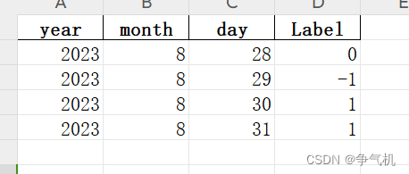
如图 , 该数据整体是一个有序的时间序列 , Label记录了每一天的状态标签 , 共三种状态.
目的 : 该demo的目的是根据该时间序列和标签预测未来某天的状态标签.
代码、注释、方法描述、问题(训练):
直接抛出代码
1、导入包
其中common为训练工具包,我会放出部分代码
import pandas as pd
from sklearn.neural_network import MLPClassifier
import common as cmn
from sklearn.model_selection import train_test_split
2、读取文件数据
# 一、读取数据
filename = 'mydata02.xlsx'
# 参数header能够指定文件的哪一行作为文件数据的列名
sheet = 'sheet1'
df = pd.read_excel(filename, sheet, header=0)
这里读取excel文件的方法参数学习借鉴,这里详细介绍了pd.read_excel()的各项参数: pandas数据处理:常用却不甚了解的函数,pd.read_excel() (baidu.com)
3、数据标准化
# 1)特征标识
target = 'Label'
# pos_label = ''  #这个值用于二分类,该demo为三分类
# 获取数据列名,并将其转换为列表格式
cols = df.columns.tolist()
# 移除标签列
cols.remove(target)
# 2)数值标准化
# 神经网络对特征的量纲比较敏感,所以要先标准化处理
from sklearn.preprocessing import StandardScaler
enc = StandardScaler()    # 实例化一个标准化对象
df[cols] = enc.fit_transform(df[cols]) # 标准化特征值
4、构建网络模型
# 定义模型
from sklearn.neural_network import MLPClassifier
mdl = MLPClassifier(
    hidden_layer_sizes=(5,5),    #隐含层
    activation='relu',        #激活函数
    solver='lbfgs',            #优化器
    learning_rate_init=0.001,    #初始化学习率
    learning_rate='adaptive',    #学习率更新方法

    #优化算法中止的条件。当迭代先后的函数差值小于等于tol时就中止
    tol=0.0001,
    max_iter=3000,                #最大迭代次数
    random_state=1                #随机种子
)
# 对网络进行训练,model_fit_clf()在common.py里
model = cmn.model_fit_clf(mdl, df, cols, target, test_size=0.2)
5、common.py
这是一个训练相关的封装包
方法 model_fit_clf()
# 训练并且评估模型
def model_fit_clf(model:BaseEstimator, df:pd.DataFrame, cols:str, target:str, labels= None, pos_label=None, test_size= 0.3, validation_size= None):
    # 划分数据集
    if test_size is None:
        X_train = df[cols]
        y_train = df[target]
    else:
        X_train, X_test, y_train, y_test = train_test_split(df[cols], df[target], test_size=test_size, random_state=0)

    # 验证集
    if validation_size is not None:
        X_train, X_validation, y_train, y_validation = train_test_split(X_train, y_train, test_size=validation_size, random_state=0)

    # 训练模型
    if validation_size is not None:
        model.fit(X_train, y_train, eval_set= [(X_validation, y_validation)])
    else:
        model.fit(X_train, y_train )

    # 评估模型
    # pred是预测出来的标签
    pred = model.predict(X_train)
    # 显示各项指标
    displayClassifierMetrics(y_train, pred, labels, pos_label)

    # probs应该是预测出来的值
    probs = model.predict_proba(X_train)
    displayROCurve(y_train, probs, labels)

    if test_size is not None:
        # 这里是测试的数据
        pred = model.predict(X_test)
        displayClassifierMetrics(y_test, pred, labels, pos_label)
        probs = model.predict_proba(X_test)
        displayROCurve(y_test, probs, labels)
方法 displayROCurve()
from sklearn import metrics
# 显示ROC曲线和AUC值
def displayROCurve(y_true:np.ndarray, y_probs:np.ndarray, labels=None, title='ROC曲线'):
    '''
    功能:  绘制ROC曲线,以及计算AUC值.
    参数:  y_true:真实值数组
            y_probs:各类别的概率矩阵
            labels:标签列表
    返回:  无
    '''
    lbls = list(np.unique(y_true))
    if labels is None:
        labels = lbls
    nPlot = len(lbls)  #子图个数
    for pos, label in enumerate(lbls):
        # 计算相关指标
        fpr, tpr, _ = metrics.roc_curve(y_true, y_probs[:,pos], pos_label=[label])
        # pos_label正类的标签,默认为None(即1)
        auc = metrics.auc(fpr, tpr)     #AUC,利用fpr, tpr计算
        # auc = metrics.roc_auc_score(y_true, y_prob[:,pos])

        plt.subplot(1, nPlot, pos+1)
        plt.plot(fpr, tpr, label='{}'.format(labels[pos]))
        plt.plot([0,1], [0,1], linestyle='--', color='k', label='random')
        plt.text(0, 1, "AUC={0:.6f}".format(auc))
        plt.legend(loc='lower right')

        plt.xlabel('False Positive Rate')
        plt.ylabel('True Positive Rate')

    plt.suptitle(title)
    plt.show()

    return
方法 displayClassifierMetrics()
def displayClassifierMetrics(y_true:np.ndarray, y_pred:np.ndarray, labels:list=None, pos_label=None):
    '''
    功能:  计算分类模型的混淆矩阵,以及评估指标.
    参数:  y_true:真实值数组
            y_pred:预测值数组
            labels:标签名称
            pos_label:正类标签, 此值必须出现在labels中, 二分类时使用。
    返回:混淆矩阵,评估指标字典。即(dfMatrix, mts)
    '''

    # 获取混淆矩阵
    matrix = metrics.confusion_matrix(y_true, y_pred)
    #去除一维数组或列表中的重复元素,返回新的无元素重复的元组或者列表
    lbls = list(np.unique([y_true, y_pred]))
    dfMatrix = pd.DataFrame(matrix, columns=lbls, index=lbls)

    if labels is not None:
        labels = list(labels)

        dct = dict(zip(lbls, labels))
        dfMatrix.rename(dct, axis=0, inplace=True)
        dfMatrix.rename(dct, axis=1, inplace=True)
    else:
        labels = lbls

    if pos_label is None:
        pos_label = labels[-1]      #默认最后一个为正类
    pos_lbl = lbls[labels.index(pos_label)]

    #给混淆矩阵添上sum行和列
    sum_label = 'sum'
    dfMatrix.loc[sum_label] = dfMatrix.sum(axis=0)
    dfMatrix[sum_label] = dfMatrix.sum(axis=1)

    print(dfMatrix, '\n')

    # 计算评估指标
    if len(lbls) <= 2:  #二分类
        mts = {}
        mts['Accuracy'] = metrics.accuracy_score(y_true, y_pred)   #正确率

        # pos_label = lbls[labels.index(pos_label)]

        mts['Precision'] = metrics.precision_score(y_true, y_pred,labels=lbls,pos_label=pos_lbl,average='binary')
        mts['Recall'] =  metrics.recall_score(y_true, y_pred,labels=lbls,pos_label=pos_lbl,average='binary')

        neg_num = dfMatrix.loc[sum_label,sum_label]-dfMatrix.loc[pos_label, sum_label]
        fp_num = dfMatrix.loc[sum_label, pos_label] - dfMatrix.loc[pos_label, pos_label]
        mts['Specificity'] =  1- fp_num /neg_num

        mts['F1'] =  metrics.f1_score(y_true, y_pred, labels=lbls, pos_label=pos_lbl,average='binary')
        mts['Lift'] =  mts['Recall']/(dfMatrix.loc[pos_label, sum_label] / dfMatrix.loc[sum_label,sum_label])

        # 格式化一下,保留4位小数
        for k,v in mts.items():
            mts[k] = np.round(v, 4)
        print(mts)

    else:
        dfclfMetric = pd.DataFrame(index=['Accuracy', 'Precision', 'Recall', 'F1'], dtype= 'float')

        dfclfMetric.loc['Accuracy', 'macro'] = metrics.accuracy_score(y_true, y_pred)
        for avg in ['macro', 'micro']:
            dfclfMetric.loc['Precision', avg] = metrics.precision_score(y_true, y_pred,labels=lbls,average=avg)
            dfclfMetric.loc['Recall', avg] = metrics.recall_score(y_true, y_pred,labels=lbls,average=avg)
            dfclfMetric.loc['F1', avg] = metrics.f1_score(y_true, y_pred,labels=lbls,average=avg)

        print(dfclfMetric.round(4))     #保留4位小数

    return
模型训练后预测使用
test_date = {"year": [2023, 2023, 2023, 2023, 2023, 2023], "month": [8, 8, 8, 8, 9, 9], "day": [28, 29, 30, 31, 21, 20]}
# 转换数据格式
test_date = pd.DataFrame(test_date)
# 获取训练集的均值和标准差
mean=enc.mean_    #均值
scale=enc.scale_    #标准差
#标准化
test_date=test_date-mean
test_date=test_date/scale
print(model.predict(test_date))    #打印预测结果


 1万+
1万+


 被折叠的 条评论
为什么被折叠?
被折叠的 条评论
为什么被折叠?
 到【灌水乐园】发言


