机器学习——Naive Bayes算法

学习来源： NB 算法 (包括符号型与数值型, 结合 Java 程序分析)
日撸 Java 三百行（51-60天，kNN 与 NB）

前言：Naive Bayes 是一个经典的、有代表性的分类算法. Naive 的 i 上面应该是两个点, 它读作 “哪义乌”, 表示很傻瓜很天真.

一、符号型数据的Naive Bayes算法

1.例子数据集

可在 https://gitee.com/fansmale/javasampledata 下载.

@relation weather.symbolic

@attribute outlook {sunny, overcast, rainy}
@attribute temperature {hot, mild, cool}
@attribute humidity {high, normal}
@attribute windy {TRUE, FALSE}
@attribute play {yes, no}

@data
sunny,hot,high,FALSE,no
sunny,hot,high,TRUE,no
overcast,hot,high,FALSE,yes
rainy,mild,high,FALSE,yes
rainy,cool,normal,FALSE,yes
rainy,cool,normal,TRUE,no
overcast,cool,normal,TRUE,yes
sunny,mild,high,FALSE,no
sunny,cool,normal,FALSE,yes
rainy,mild,normal,FALSE,yes
sunny,mild,normal,TRUE,yes
overcast,mild,high,TRUE,yes
overcast,hot,normal,FALSE,yes
rainy,mild,high,TRUE,no

• 这里的前四列分别对应四种天气属性{outlook, temperature, humidity, windy}的不同情况，最后一列则是根据前四列的描述来决定是否出去玩，表示为{yes, no}。

2. 基础理论

2.1 条件概率

$$P(AB)=P(A)P(B\mid A)\text{\hspace{1em}(1)}$$
其中:

• P(A)表示事件 A发生的概率;
• P(AB)表示事件 A 和 B 同时发生的概率;
• P(B∣A)表示在事件 A 发生的情况下, 事件 B 也发生的概率.

例: A 表示天气是晴天, 即 outlook = sunny; B 表示湿度高, 即 humidity = high.
14 天中, 有 5 天 sunny, 则P(A) = P(outlook = sunny) = $\frac{4}{15}$
这 5 个晴天中, 有 3 天温度高, 则 P(B∣A) = P(humidity = high | outlook = sunny)= $\frac{3}{5}$
那么, 即是晴天又温度高的概率是P(AB) = P(outlook = sunny $\wedge$ humidity= high) = $\frac{3}{14}$ = P(A)P(B∣A)

2.2 独立性假设

令 $\mathbf{x}$ = x₁ $\wedge$ x₂ $\wedge$ ⋯ $\wedge$ x_m 表示一个条件的组合, 如: outlook = sunny $\wedge$ temperature = hot $\wedge$ humidity = high $\wedge$ windy = FALSE,它对应于我们数据集的第一行.
令 D_i 表示一个事件, 如: play = no. 根据 (1) 式可知:

$$P(D_i|\mathbf{x})=\frac{P(\mathbf{x}{D}_i)}{P(\mathbf{x})}=\frac{P(D_i)P(\mathbf{x}|D_i)}{P(\mathbf{x})}\text{\hspace{1em}(2)}$$

这就是贝叶斯公式，它精妙的地方就在于对于甲事件发生条件下乙发生的条件概率可以通过倒过来的乙发生条件下甲发生的条件概率来计算！

现在我们做一个大胆的假设, 认为各个条件之间是独立的:
$$P(\mathbf{x}|D_i)=P(x_1|D_i)P(x_2|D_i)....P(x_m|D_i)=\prod _{j=1}^{m}P(x_j|D_i)\text{\hspace{1em}(3)}$$
这个大胆的假设, 就是 Naive 的来源. 在现实数据中, 它是不成立的!
综合 (2)(3) 式可得:
$$P(D_i|\mathbf{x})=\frac{P(\mathbf{x}{D}_i)}{P(\mathbf{x})}=\frac{P(D_i){\prod }_{j=1}^{m}P(x_j|D_i)}{P(\mathbf{x})}\text{\hspace{1em}(4)}$$

如果用例子替换成 P(play = no | outlook = sunny $\wedge$ temperature = hot $\wedge$ humidity = high $\wedge$ windy = FALSE),就读作: “在出太阳而且气温高而且湿度高而且没风的天气, 不打球的概率”.
这个概率是算不出来的, 因为我们计算不了分母P($\mathbf{x}$). 不过我们的目标是进行分类, 也就是说, 哪个类别的概率高, 我们就选谁. 而对不同的类别, 这个式子的分母是完全相同的!
所以我们的预测方案就可以描述为:

• d($\mathbf{x}$)表示的是当前最佳决策属性的下标，比如在weather数据集中最佳决策属性是一个长度为2的数组，Judge[0]表示不去玩，Judge[1]表示去玩，当返回的d($\mathbf{x}$)=1时就是去玩。
• argmax 表示哪个类别的相对概率高, 我们就预测为该类别.

(5)式中有大量概率相乘的情况，因为这里概率都是小于1的，所以最终的结果可能是一个非常小的数，对于计算机来说，这存在越界风险。于是我们可以通过log运算放大这个结果，同时因为log是单调递增的函数，对于多个要比大小的数据来说，这并不改变数据相互的大小关系.

2.3 Laplacian 平滑

上面的log代替合理吗？log的定义域是(0,+∞)，而一般的概率范围是[0,+∞)。发现危险了吗？

(5) 式在预测时会出现问题. 例如:

• P(outlook = overcast | play = no) = 0, 即不打球的时候, 天气不可能是多云. 如果新的一天为阴天, 则不打球的概率为 0.
• P(temperature = hot | play = yes) = 0, 即打球的时候, 温度不可能是高. 如果新的一天温度高, 则打球的概率为 0.
  那么, 如果有一天 outlook = overcast $\wedge$ temperature = hot, 岂不是打球和不打球的概率都为 0 了?
  这里的根源在于 “一票否决权”, 即 (5) 式的连乘因子中, 只要有一个为 0, 则乘积一定为 0. 为了解决该问题, 我们要想办法让这个因子不要取 0 值.
  
  其中, n 是对象的数量,v_j是第 j 个属性的可能取值数, outlook 有 3 种取值. 这样可以保证
• $P^L(x_j|D_i)>0$;
• outlook 三种取值导致的条件概率之和恒为 1. 即
  $$P^L(outlook=sunny|play=yes)+P^L(outlook=overcast|play=yes)+P^L(rain=sunny|play=yes)=1.$$
  对于$P(D_i)$也需要进行平滑:
  $$P^L(D_i)=\frac{nP(D_i)+1}{n+c}\text{\hspace{1em}(8)}$$

考虑 Laplacian 平滑的优化目标为:

二、数值型数据的Naive Bayes算法

1.例子数据集

@RELATION iris
 
@ATTRIBUTE sepallength	REAL
@ATTRIBUTE sepalwidth 	REAL
@ATTRIBUTE petallength 	REAL
@ATTRIBUTE petalwidth	REAL
@ATTRIBUTE class 	{Iris-setosa,Iris-versicolor}
 
@DATA
5.1,3.5,1.4,0.2,Iris-setosa
4.9,3.0,1.4,0.2,Iris-setosa
4.7,3.2,1.3,0.2,Iris-setosa
4.6,3.1,1.5,0.2,Iris-setosa
5.0,3.6,1.4,0.2,Iris-setosa
5.4,3.9,1.7,0.4,Iris-setosa
4.6,3.4,1.4,0.3,Iris-setosa
5.0,3.4,1.5,0.2,Iris-setosa
...
6.9,3.1,4.9,1.5,Iris-versicolor
5.5,2.3,4.0,1.3,Iris-versicolor
6.5,2.8,4.6,1.5,Iris-versicolor
5.7,2.8,4.5,1.3,Iris-versicolor
6.3,3.3,4.7,1.6,Iris-versicolor
4.9,2.4,3.3,1.0,Iris-versicolor
6.6,2.9,4.6,1.3,Iris-versicolor
5.2,2.7,3.9,1.4,Iris-versicolor
5.0,2.0,3.5,1.0,Iris-versicolor
...

2. 算法理论

• 脱离了离散概率的特性，我们的概率表示应当是随机变量的区间，即假设对于第一列，sepallength为5.0的概率我可以使用$P4.9\le sepallength<5.1$.但是针对离散的点集使用这种连续处理太过于麻烦了，于是我们进一步简化这个过程。
• 因为最终我们都是比对这些概率条件下的大小问题，因此我们可以让所有的数据列都适用一种概率评价指标。假设对于某个属性列$\mathrm{X}$（随机变量），存在一个离散值x。这时我们设法将概率计算的区间缩小到足够小的范围$\sigma$（$\sigma$>0）
• 因为$\sigma$足够小，以至于曲线近似于直线，这样的话，概率密度函数的每个小的曲边梯形面积可以近似表示为$\sigma p(x)$。由于对于所有的概率比对来说，都有σ这个固定系数，因此可以同时忽略。这样的话，对于某个数值型的离散概率比较，近似地可以用概率密度函数$p(x)$来度量。

这里可以假设服从正态分布，这种假设对于通常的未知数据是可靠的，稳定的。因此我们得到了数值型的离散数据的概率计算公式：

字符型数据的Naive Bayes公式在未经过Laplacian平滑的环境下的公式：

这里（2）式中的$P^L(x_j\mid D_i)$拿出来，这里含义是在$D_i$决策下对于$x_j$属性列的概率计算，转化为数值型之后，这里的$x_j$列管辖的所有元素都是确定的数值而非字符了，因此可以计算出确定的在$D_i$条件下的${\mu }_j$，即${\mu }_{ij}$，同理也有${\sigma }_{ij}$。但是上式中的$P^L(D_i)$并不需要代替，因为无论是数值型问题还是字符型问题，我们的决策结果总是一个确定的分类描述，这个描述是字符型的，这个是由我们研究的分类问题本质决定的。回归问题研究决策信息才是连续的数值。综上，用$p(x_j)$来代表（2）式中的$P^L(x_j\mid D_i)$，从而得到下面的式子：

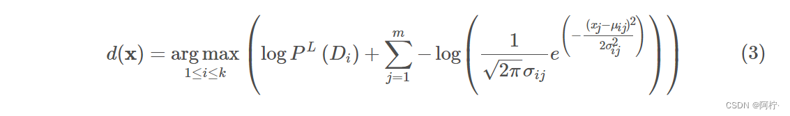
这个3式可以化简，首先在共同求最大值的操作中，正的常系数$\frac{1}{\sqrt{2\pi }}$是可以忽略的，因为同时除这个系数不影响全局的大小关系。此外，将内部的指数运算同外部的log结合，因此得到最终表达式：

这里的 ${\sigma }_{ij}$ 和${\mu }_{ij}$表示方差与均值，都与类别和属性相关.

这个式子就是数值型Naive Bayes的推导式了，因为一般都采用正态分布带描述一般的数值数据，而正态分布又叫做高斯分布，所以一般的数值型Naive Bayes又称之为Gaussian Naive Bayes算法。

三、实现代码

package machinelearning.bayes;

import java.io.FileReader;
import java.util.Arrays;

import weka.core.Instance;
import weka.core.Instances;

/**
 * 
 * @author Ling Lin E-mail:linling0.0@foxmail.com
 * 
 * @version 创建时间：2022年5月8日 下午9:43:08
 * 
 */
public class NaiveBayes {

	/**
	 * An inner class to store parameters.
	 */
	private class GaussianParamters {
		double mu;
		double sigma;

		public GaussianParamters(double paraMu, double paraSigma) {
			mu = paraMu;
			sigma = paraSigma;
		}// Of the constructor

		@Override
		public String toString() {
			return "(" + mu + ", " + sigma + ")";
		}// Of toString
	}// Of GaussianParamters

	/**
	 * The data.
	 */
	Instances dataset;

	/**
	 * The number of classes. For binary classification it is 2.
	 * 表示我们决策列具有的类别数目，就是我们公式中的k。本数据集中决策数据列只有yes与no两种情况
	 */
	int numClasses;

	/**
	 * The number of instances. 表示表的数据行个数，即公式中的n
	 */
	int numInstances;

	/**
	 * The number of conditional attributes. 条件数目，即m，是除开最后的决策列之后的常规训练的属性列。
	 */
	int numConditions;

	/**
	 * The prediction, including queried and predicted labels.
	 * 是一个长度为n预测数组，用于存放对于每一行数据进行leave-one-out测试时存放的预测结果。
	 */
	int[] predicts;

	/**
	 * Class distribution. 是公式中的P(Di)，因为我们数据集中k=2，故这个数组长度也为2
	 */
	double[] classDistribution;

	/**
	 * Class distribution with Laplacian smooth. 是公式中的
	 * P^L^(Di)，因为我们数据集中k=2，故这个数组长度也为2
	 */
	double[] classDistributionLaplacian;

	/**
	 * To calculate the conditional probabilities for all classes over all
	 * attributes on all values.
	 * 
	 * conditionalCounts[i][j][k]表示采用第i个决策（这里代表yes or no）， 并且当天的天气的第j种特征为第k种的数目。
	 */
	double[][][] conditionalCounts;

	// The conditional probabilities with Laplacian smooth.
	// 表示P^L^(xjDi)
	double[][][] conditionalProbabilitiesLaplacian;

	// The Guassian parameters.
	GaussianParamters[][] gaussianParameters;

	// 设置适用于什么类型的NB算法，0表示字符型，1表示的数值型
	int dataType;

	// Nominal.
	public static final int NOMINAL = 0;

	// Numerical.
	public static final int NUMERICAL = 1;

	/**
	 * The constructor.
	 * 
	 * @param paraFilename
	 *            The given file. 构造函数主要完成数据的输入，确定决策类，然后逐次给类中对应公式的n、m、k初始化。
	 */
	public NaiveBayes(String paraFilename) {
		dataset = null;
		try {
			FileReader fileReader = new FileReader(paraFilename);
			dataset = new Instances(fileReader);
			fileReader.close();
		} catch (Exception ee) {
			System.out.println("Cannot read the file: " + paraFilename + "\r\n" + ee);
			System.exit(0);
		} // Of try

		dataset.setClassIndex(dataset.numAttributes() - 1);
		numConditions = dataset.numAttributes() - 1;// m
		numInstances = dataset.numInstances();// n
		numClasses = dataset.attribute(numConditions).numValues();// k
	}// Of the constructor

	/**
	 * Set the data type.
	 */
	public void setDataType(int paraDataType) {
		dataType = paraDataType;
	}// Of setDataType

	/**
	 * Calculate the class distribution with Laplacian smooth. 计算P^L^(Di)
	 */
	public void calculateClassDistribution() {
		classDistribution = new double[numClasses];
		classDistributionLaplacian = new double[numClasses];

		// 统计对应的决策列属性出现的次数，也就是频度
		double[] tempCounts = new double[numClasses];
		for (int i = 0; i < numInstances; i++) {
			int tempClassValue = (int) dataset.instance(i).classValue();
			tempCounts[tempClassValue]++;
		} // Of for i

		for (int i = 0; i < numClasses; i++) {
			// 计算P(Di)
			classDistribution[i] = tempCounts[i] / numInstances;
			// 计算P^L^(Di)的化简公式
			classDistributionLaplacian[i] = (tempCounts[i] + 1) / (numInstances + numClasses);
		} // Of for i

		System.out.println("Class distribution: " + Arrays.toString(classDistribution));
		System.out.println("Class distribution Laplacian: " + Arrays.toString(classDistributionLaplacian));
	}// Of calculateClassDistribution

	/**
	 * Calculate the conditional probabilities with Laplacian smooth. ONLY scan
	 * the dataset once. There was a simpler one, I have removed it because the
	 * time complexity is higher.
	 * 
	 * 计算P^L^(xjDi)
	 */
	public void calculateConditionalProbabilities() {
		// 没有给出第三个维的初始化，这是因为第三维度是对应非决策列能表示的不同类别个数，
		// 这个是随不同列而不同的，因此无法确定
		conditionalCounts = new double[numClasses][numConditions][];
		conditionalProbabilitiesLaplacian = new double[numClasses][numConditions][];

		// Allocate space
		for (int i = 0; i < numClasses; i++) {
			for (int j = 0; j < numConditions; j++) {
				int tempNumValues = dataset.attribute(j).numValues();
				conditionalCounts[i][j] = new double[tempNumValues];
				conditionalProbabilitiesLaplacian[i][j] = new double[tempNumValues];
			} // Of for j
		} // Of for i

		// Count the numbers
		int[] tempClassCounts = new int[numClasses];
		for (int i = 0; i < numInstances; i++) {
			int tempClass = (int) dataset.instance(i).classValue();
			// 统计不同决策的频度
			tempClassCounts[tempClass]++;

			for (int j = 0; j < numConditions; j++) {
				int tempValue = (int) dataset.instance(i).value(j);
				conditionalCounts[tempClass][j][tempValue]++;
			} // Of for j
		} // Of for i

		// Now for the real probability with Laplacian
		// P^L^(xjDi)
		for (int i = 0; i < numClasses; i++) {
			for (int j = 0; j < numConditions; j++) {
				int tempNumValues = dataset.attribute(j).numValues();
				for (int k = 0; k < tempNumValues; k++) {
					conditionalProbabilitiesLaplacian[i][j][k] = (conditionalCounts[i][j][k] + 1)
							/ (tempClassCounts[i] + tempNumValues);
				} // Of for k
			} // Of for j
		} // Of for i

		System.out.println("Conditional probabilities: " + Arrays.deepToString(conditionalCounts));
	}// Of calculateConditionalProbabilities

	/**
	 * Calculate the conditional probabilities with Laplacian smooth.
	 	计算μij 与σij
	 */
	public void calculateGausssianParameters() {
		gaussianParameters = new GaussianParamters[numClasses][numConditions];

		double[] tempValuesArray = new double[numInstances];
		int tempNumValues = 0;
		double tempSum = 0;

		for (int i = 0; i < numClasses; i++) {
			for (int j = 0; j < numConditions; j++) {
				tempSum = 0;

				// Obtain values for this class.
				tempNumValues = 0;
				for (int k = 0; k < numInstances; k++) {
					if ((int) dataset.instance(k).classValue() != i) {
						continue;
					} // Of if

					tempValuesArray[tempNumValues] = dataset.instance(k).value(j);
					tempSum += tempValuesArray[tempNumValues];
					tempNumValues++;
				} // Of for k

				// Obtain parameters.
				double tempMu = tempSum / tempNumValues;

				double tempSigma = 0;
				for (int k = 0; k < tempNumValues; k++) {
					tempSigma += (tempValuesArray[k] - tempMu) * (tempValuesArray[k] - tempMu);
				} // Of for k
				tempSigma /= tempNumValues;
				tempSigma = Math.sqrt(tempSigma);

				gaussianParameters[i][j] = new GaussianParamters(tempMu, tempSigma);
			} // Of for j
		} // Of for i

		System.out.println(Arrays.deepToString(gaussianParameters));
	}// Of calculateGausssianParameters

	/**
	 ********************
	 * Classify all instances, the results are stored in predicts[].
	 ********************
	 */
	public void classify() {
		predicts = new int[numInstances];
		for (int i = 0; i < numInstances; i++) {
			predicts[i] = classify(dataset.instance(i));
		} // Of for i
	}// Of classify

	/**
	 ********************
	 * Classify an instances.
	 ********************
	 */
	public int classify(Instance paraInstance) {
		if (dataType == NOMINAL) {
			return classifyNominal(paraInstance);
		} else if (dataType == NUMERICAL) {
			return classifyNumerical(paraInstance);
		} // Of if

		return -1;
	}// Of classify

	/**
	 * Classify an instances with nominal data.
	 */
	public int classifyNominal(Instance paraInstance) {
		// Find the biggest one
		double tempBiggest = -10000;
		int resultBestIndex = 0;
		for (int i = 0; i < numClasses; i++) {
			double tempClassProbabilityLaplacian = Math.log(classDistributionLaplacian[i]);
			double tempPseudoProbability = tempClassProbabilityLaplacian;
			for (int j = 0; j < numConditions; j++) {
				int tempAttributeValue = (int) paraInstance.value(j);

				// Laplacian smooth.
				tempPseudoProbability += Math.log(conditionalCounts[i][j][tempAttributeValue])
						- tempClassProbabilityLaplacian;
			} // Of for j

			if (tempBiggest < tempPseudoProbability) {
				tempBiggest = tempPseudoProbability;
				resultBestIndex = i;
			} // Of if
		} // Of for i

		return resultBestIndex;
	}// Of classifyNominal

	/**
	 ********************
	 * Classify an instances with numerical data.
	 ********************
	 */
	public int classifyNumerical(Instance paraInstance) {
		// Find the biggest one
		double tempBiggest = -10000;
		int resultBestIndex = 0;

		for (int i = 0; i < numClasses; i++) {
			double tempClassProbabilityLaplacian = Math.log(classDistributionLaplacian[i]);
			double tempPseudoProbability = tempClassProbabilityLaplacian;
			for (int j = 0; j < numConditions; j++) {
				double tempAttributeValue = paraInstance.value(j);
				double tempSigma = gaussianParameters[i][j].sigma;
				double tempMu = gaussianParameters[i][j].mu;

				tempPseudoProbability += -Math.log(tempSigma)
						- (tempAttributeValue - tempMu) * (tempAttributeValue - tempMu) / (2 * tempSigma * tempSigma);
			} // Of for j

			if (tempBiggest < tempPseudoProbability) {
				tempBiggest = tempPseudoProbability;
				resultBestIndex = i;
			} // Of if
		} // Of for i

		return resultBestIndex;
	}// Of classifyNumerical

	/**
	 ********************
	 * Compute accuracy.
	 ********************
	 */
	public double computeAccuracy() {
		double tempCorrect = 0;
		for (int i = 0; i < numInstances; i++) {
			if (predicts[i] == (int) dataset.instance(i).classValue()) {
				tempCorrect++;
			} // Of if
		} // Of for i

		double resultAccuracy = tempCorrect / numInstances;
		return resultAccuracy;
	}// Of computeAccuracy

	/**
	 ************************* 
	 * Test nominal data.
	 ************************* 
	 */
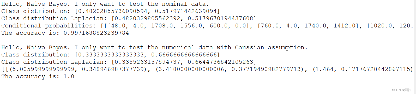
	public static void testNominal() {
		System.out.println("Hello, Naive Bayes. I only want to test the nominal data.");
		String tempFilename = "D:/00/data/mushroom.arff";

		NaiveBayes tempLearner = new NaiveBayes(tempFilename);
		tempLearner.setDataType(NOMINAL);
		tempLearner.calculateClassDistribution();
		tempLearner.calculateConditionalProbabilities();
		tempLearner.classify();

		System.out.println("The accuracy is: " + tempLearner.computeAccuracy());
	}// Of testNominal

	/**
	 ************************* 
	 * Test numerical data.
	 ************************* 
	 */
	public static void testNumerical() {
		System.out.println("Hello, Naive Bayes. I only want to test the numerical data with Gaussian assumption.");
		// String tempFilename = "D:/data/iris.arff";
		String tempFilename = "D:/00/data/iris-imbalance.arff";

		NaiveBayes tempLearner = new NaiveBayes(tempFilename);
		tempLearner.setDataType(NUMERICAL);
		tempLearner.calculateClassDistribution();
		tempLearner.calculateGausssianParameters();
		tempLearner.classify();

		System.out.println("The accuracy is: " + tempLearner.computeAccuracy());
	}// Of testNominal

	/**
	 ************************* 
	 * Test this class.
	 * 
	 * @param args
	 *            Not used now.
	 ************************* 
	 */
	public static void main(String[] args) {
		testNominal();
		System.out.println();
		testNumerical();
	}// Of main
}// Of class NaiveBayes