Artificial Intelligence -- Chapter 9 Hidden Markov Models

We can't observe states, but we can observe some indirect evidence about the states, and we will use these evidence to infer what the state is like. (We see E, and we infer X by E)

Now we have an observation model, this is the information about what we expect to see given our environment in a certain state. We can see the model is the form the probability of an observation/ evidence given that the environment is in a certain state.

Just like what's shown in the graph, X1 leads to E1, X2 leads to E2...

At each time step, we're going to be able to observe whether or not someone is taking an umbrella. We should know that taking an umbrella doesn't mean it's rainy.

Here the observation model indicates the probability of observing an umbrella or not given that it's rainy or not.

For this question, we are going to compute given Et, what's the probability of Xt

Now firstly we consider a purely Markov chain. So we have:

Then we actually observe evidence:

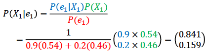
Note that

• P(X1| E1) = P(X1| e1) = P(X1| +u)
• P(e1) = P(e1,+r)+P(e1,-r) = P(e1| +r) P(+r) + P(e1| -r) P(-r)  Marginalization and Product rule
• Now we have an observation for each step, then the property of the initial state is insignificant still hold in this case, but the property of convergence will not hold (the stationary distribution not hold)

Recall that the immediate predecessor cuts off all the previous states from the state in the future. It still holds in Hidden Markov Models (HMM): given a preceding state, nothing in the past matters. It means, if you're telling me the value of a specific state, that is enough information for me to determine what happens in the next state regardless of whatever happened before.

For example, in the graph, we say given X3, what is X4 like has no relation with X1,E1,X2,E2,E3. It's just the meaning of the transition model P(Xt | Xt-1)

Another independent statement is: given the current state, its observation variable Et is conditionally independent of all past states and evidence as well. 

In the graph, if we know the state X4, then it's enough to determine what E4 looks like. It's obvious since it's the definition of the observation model P(Et | Xt)

So in HMM, we have conditionally independence on both state and observation.

Using the above two statement for conditionally independence:

P(X1,E1,X2,E2,X3,E3,...) 

= P(X1) P(E1|X1) P(X2|X1,E1) P(E2|X1,E1,X2) P(X3|X1,E1,X2,E2) P(E3|X1,E1,X2,E2,X3) ...

= P(X1) P(E1|X1) P(X2|X1,E1) P(E2|X1,E1,X2) P(X3|X1,E1,X2,E2) P(E3|X1,E1,X2,E2,X3) ...

= P(X1) P(E1|X1) P(X2|X1) P(E2|X2) P(X3|X2) P(E3|X3) ...

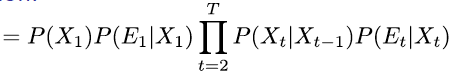
And recall that if we know P(X1,E1,X2,E2,X3,E3,...), we can extract any RVs like P(X1) or P(E1) just by marginaliztion.

Filtering is returning a probability distribution of a state.

Most likely explanation is returning a sequence of actual states.

Smoothing is also returning a distribution of a state, and we are not going to talk about this method here.

Let's see the detail of Filtering first.

• we have 22 cells, but we don't know which cell is the robot in.
• for t=0, every cell is in the same grayscale (an uniform distribution), it means that the robot  is equally possible to stay in every cell in the beginning.
• The sensor is giving a 4-bit binary string like in the red, (1010) for (North,East,South,West), 1 is for wall for the corresponding direction, and 0 is for clear/no wall. (1010) is the true value, we might have at most 1 bit error.

Now assume the robot now make an observation on its current grid and the true observation value on that grid is (1010), in this case, we can eliminate the possibility of the robot is in some certain states.

For example, the grid A has the true observation value of (1001), compared with (1010), there are two bits error. Note that the senso