数字信号处理DFS与DTFT关系

No_one-_-2022

于 2022-11-29 19:36:47 发布

阅读量571

点赞数 1

分类专栏： DSP数字信号处理文章标签：深度优先信号处理算法

本文链接：https://blog.csdn.net/m0_51143578/article/details/128103548

版权

DSP数字信号处理专栏收录该内容

10 篇文章 5 订阅

订阅专栏

一、用MATLAB编写DFS计算程序

二、寻找DFT和DTFT之间的关系

三、备注 DFS和DTFT求解公式

一、用MATLAB编写DFS计算程序

The syntax is ‘y=dfs(x, k)’, where the output vector ‘y’ represents the Fourier coefficients Ck , the input vector ‘x’ represents one period of x[n], and the parameter vector ‘k’ is the indexes in Ck .

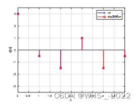
Use your ‘dfs’ function to calculate the DFS of $x[n]=2 \cos \left(\frac{2 \pi}{3} n\right)+\cos \left(\frac{\pi}{3} n\right)$ ,then use the same ‘dfs’ function to perform the inverse transform, the result $x_{1}[n]$ should be equal to $x[n]$ .

答案如下所示：

N=6; n=0:N-1;
xn =2*cos(2*pi/3*n)+cos(pi/3*n)
y=dfs(xn,n);							 %x[n]的dfs结果
x1n=dfs(y/N,-n);						 %利用函数dfs求解x[n]
amX=abs(y);angX=angle(y);				 %求解幅度及相位
angX(amX<0.001)=0;					 %将幅度为0的相位置零
angX(angX<0.001)=0;					 %将很小的相位置零
function y=dfs(x,k)						 %dfs函数实现
    N=length(k);
    n=0:N-1;
    y=x*exp(-j*2*pi/N).^(n'*k);
end

二、寻找DFT和DTFT之间的关系

A nonperiodic sequence $x_{1}[n]=u[n]-u[n-4]$ ,use your own ‘dtft’ function to find out the spectrum. A periodic sequence $x_{2}[n]$ is the periodic extension of $x_{1}[n]$ . $x_{2}[n]=\sum_{k=-\infty}^{\infty} x_{1}[n-8 k]=\sum_{k=-\infty}^{\infty}\{u[(n-8 k)]-u[(n-8 k)-4]\}$ ,use your ‘dfs’ function to find out the spectrum.

Analyze the relationship between the two spectra, including magnitude and phase spectra.

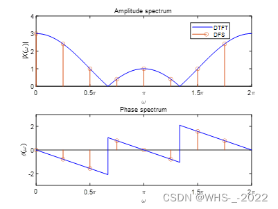
$\begin{array}{l} X_{1}(\omega)=\sum_{n=-\infty}^{\infty} R_{3}[n] e^{-j \omega n}=\sum_{n=0}^{3} e^{-j \omega n}=\frac{1-e^{-j 4 \omega}}{1-e^{-j \omega}}=\frac{e^{-j 2 \omega}\left(e^{j 2 \omega}-e^{-j 2 \omega}\right)}{e^{-j \omega / 2}\left(e^{j \omega / 2}-e^{-j \omega / 2}\right)}=e^{-j 3 \omega / 2} \frac{\sin (2 \omega)}{\sin (\omega / 2)} \\ C_{k}=\sum_{n=0}^{N-1} x_{2}[n] e^{-j 2 \pi \frac{k}{N} n}=\sum_{n=0}^{3} e^{-j 2 \pi \frac{k}{N} n}=\frac{1-e^{-j 2 \pi \frac{k}{8} \cdot 4}}{1-e^{-j 2 \pi \frac{k}{8}}}=\frac{e^{-j \frac{\pi}{2} k}\left(e^{j \frac{\pi}{2} k}-e^{-j \frac{\pi}{2} k}\right)}{e^{-j \frac{\pi}{8} k}\left(e^{j \frac{\pi}{8} k}-e^{-j \frac{\pi}{8} k}\right)}=e^{-j \frac{3 \pi}{8} k} \frac{\sin \left(\frac{\pi}{2} k\right)}{\sin \left(\frac{\pi}{8} k\right)} \end{array}$

We find that $C_{k}=X_{1}(\omega),\left(\omega=\frac{2 \pi}{N} k, N=8\right)$ ，which proves the validity of the plotting.

x=[1 1 1 1];
y1=dtft(x,[0 1 2 3]);
x2n=[1 1 1 1 0 0 0 0]
y2=dfs(x2n,[0:7]);

figure(1)
magX1=abs(y1); %绘制x(n)的幅度谱
subplot(2,1,1);plot([0:2*pi/3999:2*pi],magX1,'b');
hold on;

magX2=abs(y2); %绘制x(n)的幅度谱
subplot(2,1,1);stem([0:2*pi/8:2*pi/8*7],magX2);
xlabel('\omega'),ylabel('|\itX\rm(\omega)|');title('Amplitude spectrum');
axis([0 2*pi 0 4]);
%set(gca,'xtickmode','manual','xtick',[0,"4\pi"]);
set(gca,'xtick',[ 0  0.5*pi pi 1.5*pi 2*pi]);
xticklabels({'0','0.5\pi','\pi','1.5\pi','2\pi'})

angX1=angle(y1); %绘制x(n)的相位谱
subplot(2,1,2);plot([0:2*pi/3999:2*pi],angX1,'b');
hold on;
angX2=angle(y2); %绘制x(n)的相位谱
subplot(2,1,2);stem([0:2*pi/8:2*pi/8*7],angX2) ;xlabel('\omega'),ylabel('\it\theta\rm(\omega)'); title ('Phase spectrum');
axis([0 2*pi -3 3]);
set(gca,'xtick',[ 0  0.5*pi pi 1.5*pi 2*pi]);
xticklabels({'0','0.5\pi','\pi','1.5\pi','2\pi'})

三、备注 DFS和DTFT求解公式

function y=dfs(x,k)
    N=length(k);
    n=0:N-1
    y=x*exp(-j*2*pi/N).^(n'*k);
end
function y=dtft(x,n)
    w=linspace(0,2*pi,4000);
    y=x*exp(-j*n'*w);
end