【笔记】YOLOv7正样本匹配原理+代码（SimOTA）

主要依照个人对代码的理解。

所谓“正样本”，也就是需要计算位置损失的预测框，也可以认为是负责预测target的anchor（anchor与pred一一对应）。例如20*20，40*40，80*80三种尺寸的特征图，认为其中的anchor总数为20*20*3+40*40*3+80*80*3（等于预测框数量），从这大量anchor之中选出预测少量target的"正样本"。损失计算时（位置损失和分类损失），需要用到的是“正样本”对应的预测值与target。

一、原理

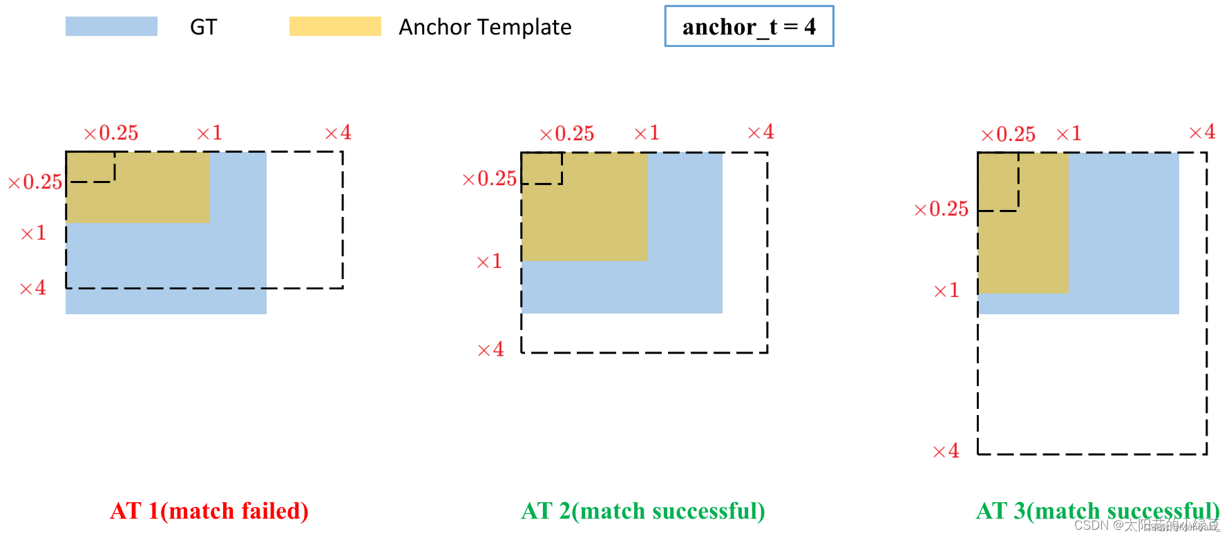
Step1. target与anchor：

真值框与9个anchor分别计算宽比（ratio_w）和高比（ratio_h），二者都介于（1/4，4）之间则认为该真值框与对应anchor匹配上。即该anchor与真值框形状大小相似，一般大部分anchor都符合，该步骤可以得到负责预测target的 0～9 个“正样本”。

图源：YOLOv5网络详解_yolov5网络结构详解-CSDN博客

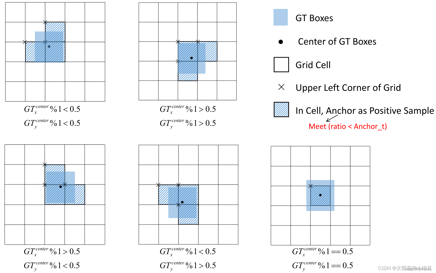
Step2. target与grid：

真值框中心点落在某grid的四个方位（左上、左下、右上、右下），则往相邻的两个方向扩展一个grid。除非精准地落在正中间，该步骤后每个target可以有3个grid负责预测，结合第一步筛选出来的anchor，可以得到负责预测该target的 0～27 个正样本。

图源：YOLOv5网络详解_yolov5网络结构详解-CSDN博客

v5以及不含OTA的v7（代码可选）到这一步就结束了。

Step3. target与IoU（SimOTA）：

需要注意，一个target可以由多个正样本预测，但一个正样本只能负责预测一个target。

（1）计算cost：计算该图像中的每个target与第二步中所有正样本对应的prediction的IoU，得到一个 nT*nP 的矩阵（其中很多值为0，因为不是该正样本负责预测的target）；同时也可以计算出IoU_cost、分类损失class_cost 以及cost = class_cost + lmd * IoU_cost。该步骤最终需得到2个 nT*nP 的矩阵IoU、cost。

（2）获取dynamic_k：对于IoU矩阵，选取与每个target的IoU最大的前10（可调，如果不足10个，有多少取多少）个pred，得到 nT*10 的矩阵；对每一行求和并向下取整，得到nT个整数，即每个target最终由多少个正样本来预测。这么做的原因是，step1,2之后，正样本个数是增多了，但鱼龙混杂，有的预测框实在太差，与target的IoU非常小，我们也把它认为是负样本，不计算损失。每一行求和得到的整数大致可以代表与这个target的IoU较大的有多少个。

（3）得到dynamic_k个正样本：对于cost矩阵，取每个target对应的前dynamic_k个预测框作为最终“正样本”。可能会遇到其中有的正样本与多个target匹配，则选取与它IoU最小的target来预测。

总结

前两步筛选出的正样本只是anchor，没有预测值也可以获得，目的是为了增加正样本数量；第三步SimOTA精细化筛选，涉及预测值，需要经过前向传播得到pred后才能计算，第1,2步的正样本anchor，给第3步提供pred索引进行初筛，再经过cost筛选，此时的“正样本”可以直接认为是接下来用来计算loss的预测框了。

注意：train.py中，通常，训练时使用加simota的正样本匹配，验证时不加。

---

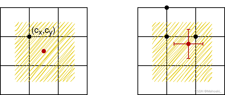
模型输出为tx, ty, tw, th，对应到实际预测框的中心点坐标以及宽高为：

可以看到中心点坐标位于(cx-0.5, cx+1.5)*(cy-0.5, cy+1.5)范围，即该grid向外扩了0.5个单位，一种解释是，若真值框中心点落在grid边界附近，原公式（v2论文给的）需要tx或ty无穷大或无穷小才能接近，对训练来说太难了，于是预测中心点可落范围向外扩了0.5个单位；

还有一种解释是，与正样本匹配第二步相呼应，若真值中心点落在(cx, cy)grid内，向邻近的两个方向扩一个grid，与中心点向上下左右四个方向分别取一个间隔0.5单位的点，这总共5个点所在的格子进行预测，效果是一样的，而从这个grid向外延伸出去的4个点，都会落在(cx-0.5, cx+1.5)*(cy-0.5, cy+1.5)范围内。

而对于宽高，原公式e^x，可能会出现梯度爆炸的问题，于是将其限制在了(0, 4)之间，而为什么是4呢，也可以理解为与上述正样本匹配的第一步宽比、高比筛选时的超参数4相呼应。

二、代码

源代码链接：https://github.com/WongKinYiu/yolov7

正样本匹配部分主要看 utils/loss.py/class ComputeLossOTA/__call__()中的一个函数build_targets()，接下来具体看一下build_targets()。

1、find_3_positive()

该函数对应原理中的前两步，也是class ComputeLoss（不含OTA）中build_targets()的全部内容，意思是class ComputeLossOTA的builid_targets()中的内容主要都是SimOTA。

indices, anch = self.find_3_positive(p, targets)  # 一个batch的predictions和targets

 进到函数里面：

def find_3_positive(self, p, targets):
    # p: {list:3}, 三个尺度的输出：N*C*H*W*(5+cls), 5表示(conf,tx,ty,tw,th)
    # targets: n_targets*6, 6表示(img_index,cls_index,x,y,w,h), 其中x,y,w,h都是归一化后的

    na, nt = self.na, targets.shape[0]  # number of anchors, targets
    indices, anch = [], []
    # 用于使归一化的xywh转换到对应的网格坐标系1->number_grid
    gain = torch.ones(7, device=targets.device).long()  # normalized to grid_space gain
    # 索引，ai.shape=(na,nt)=(3,nt)，即第一行nt个0，第二行nt个1，第三行nt个2，只用于下一步append targets
    ai = torch.arange(na, device=targets.device).float().view(na, 1).repeat(1, nt)  # same as .repeat_interleave(nt)
    # targets: nt*6 --> 3*nt*7, 7 means (img,cls,x,y,w,h,anchor), anchor represents this layer's 3 anchors
    targets = torch.cat((targets.repeat(na, 1, 1), ai[:, :, None]), 2)  # append anchor indices

    g = 0.5  # bias
    off = torch.tensor([[0, 0],
                        [1, 0], [0, 1], [-1, 0], [0, -1],  # j,k,l,m
                        # [1, 1], [1, -1], [-1, 1], [-1, -1],  # jk,jm,lk,lm
                        ], device=targets.device).float() * g  # offsets

    # ---------------------------------------------one layer-----------------------------------------------------------
    for i in range(self.nl):
        anchors = self.anchors[i]  # this layers' anchors: 3*2
        gain[2:6] = torch.tensor(p[i].shape)[[3, 2, 3, 2]]  # xyxy gain

        # Match targets to anchors
        t = targets * gain  # (3,nt,7), 将xywh转换到网格坐标系下
        if nt:
            # Matches, 3 anchors vs. nt targets
            r = t[:, :, 4:6] / anchors[:, None]  # wh ratio, r.shape=(3,nt,2)
            j = torch.max(r, 1. / r).max(2)[0] < self.hyp['anchor_t']  # compare, shape=(3,nt)
            # j = wh_iou(anchors, t[:, 4:6]) > model.hyp['iou_t']  # iou(3,n)=wh_iou(anchors(3,2), gwh(n,2))
            t = t[j]  # filter, t.shape=(nPositive,7)

            # Offsets
            gxy = t[:, 2:4]  # grid xy, 从左上数(nP,7)
            gxi = gain[[2, 3]] - gxy  # inverse, 从右下数(nP,7)
            j, k = ((gxy % 1. < g) & (gxy > 1.)).T  # bool(nP,), 落在格子左半边的，格子上半边的
            l, m = ((gxi % 1. < g) & (gxi > 1.)).T  # bool(nP,), 落在格子右半边的，格子下半边的
            j = torch.stack((torch.ones_like(j), j, k, l, m))  # (5,nP)
            t = t.repeat((5, 1, 1))[j]  # (nOffset,7), nOffset=nP+nPl+nPu+nPr+nPd
            offsets = (torch.zeros_like(gxy)[None] + off[:, None])[j]  # (5,nP,2)[j]=(nOffset,2)
        else:
            t = targets[0]
            offsets = 0

        # Define
        b, c = t[:, :2].long().T  # image, class (nOffset,)
        gxy = t[:, 2:4]  # grid xy (nOffset,2)
        gwh = t[:, 4:6]  # grid wh (nOffset,2)
        gij = (gxy - offsets).long()  # (nOffset,2), 所在网格左上角坐标
        gi, gj = gij.T  # grid xy indices   # (nOffset, )

        # Append
        a = t[:, 6].long()  # anchor indices, (nOffset,)
        indices.append((b, a, gj.clamp_(0, gain[3] - 1), gi.clamp_(0, gain[2] - 1)))  # image, anchor, grid indices
        anch.append(anchors[a])  # anchors
    # ---------------------------------------------end layer----------------------------------------------------------- 

    return indices, anch  # both {list:3}, indices[0]:{tuple:4}, anch[0]:{nOffset,2}

主要经过matches和offsets两次筛选。经过step1. matches长比宽比阈值筛选，targets变为 nPositive*7；经过step2. offsets向外扩展2个grid，targets变为nOffset*7。一般nOffset=3*nPositive。

return的indices是按layer分的{list:3}，可理解为是正样本索引[img, anch, gj, gi]，包含从 t 中获取的image_index(nOffset,)，anchor_index(nOffset,)，gj(nOffset,)，gi(nOffset,)；

anch也是按layer分开的{list:3}，储存anchor_index对应的每个anchor的尺寸。

2、build_targets()

作者主要定义了两种用来储存的变量 matching_, all_。all_用来储存一张image的信息，matching_按照layer，储存一个batch的信息，最终返回matching_用于计算损失。

def build_targets(self, p, targets, imgs):
    # input batch_predictions, batch_labels(), batch_images
    # indices, anch = self.find_positive(p, targets)
    indices, anch = self.find_3_positive(p, targets)
    # indices, anch = self.find_4_positive(p, targets)
    # indices, anch = self.find_5_positive(p, targets)
    # indices, anch = self.find_9_positive(p, targets)
    device = torch.device(targets.device)
    matching_bs = [[] for pp in p]
    matching_as = [[] for pp in p]
    matching_gjs = [[] for pp in p]
    matching_gis = [[] for pp in p]
    matching_targets = [[] for pp in p]
    matching_anchs = [[] for pp in p]

    nl = len(p)
    # ------------------------------------------one image in the batch---------------------------------------------
    for batch_idx in range(p[0].shape[0]):
        b_idx = targets[:, 0] == batch_idx  # 取该图像编号对应的targets
        this_target = targets[b_idx]  # nt_of_this_img * 6
        if this_target.shape[0] == 0:
            continue

        txywh = this_target[:, 2:6] * imgs[batch_idx].shape[1]  # 转换到像素坐标系(640*640)
        txyxy = xywh2xyxy(txywh)  # --> 左上右下顶点坐标

        pxyxys = []
        p_cls = []
        p_obj = []
        from_which_layer = []
        all_b = []
        all_a = []
        all_gj = []
        all_gi = []
        all_anch = []

        # ------------------------------------one layer of the image prediction------------------------------------
        for i, pi in enumerate(p):  # pi: N*C*H*W*(5+cls)
            b, a, gj, gi = indices[i]  # 这一层的正样本索引[b,a,gj,gi]
            idx = (b == batch_idx)
            b, a, gj, gi = b[idx], a[idx], gj[idx], gi[idx]  # 这一层中对应该图像的正样本索引
            all_b.append(b)
            all_a.append(a)
            all_gj.append(gj)
            all_gi.append(gi)
            all_anch.append(anch[i][idx])
            from_which_layer.append((torch.ones(size=(len(b),)) * i).to(device))

            # 根据索引获取正样本预测值
            fg_pred = pi[b, a, gj, gi]  # nPositive*85
            p_obj.append(fg_pred[:, 4:5])
            p_cls.append(fg_pred[:, 5:])

            # 计算预测框实际位置(像素坐标系, 640*640)
            grid = torch.stack([gi, gj], dim=1)
            pxy = (fg_pred[:, :2].sigmoid() * 2. - 0.5 + grid) * self.stride[i]  # / 8.
            # pxy = (fg_pred[:, :2].sigmoid() * 3. - 1. + grid) * self.stride[i]
            pwh = (fg_pred[:, 2:4].sigmoid() * 2) ** 2 * anch[i][idx] * self.stride[i]  # / 8.
            pxywh = torch.cat([pxy, pwh], dim=-1)
            pxyxy = xywh2xyxy(pxywh)  # nPositive*4
            pxyxys.append(pxyxy)  # list, append 3 layers' pxyxy
            # ------------------------------------------end layer--------------------------------------------------

        # three layers appended, pxyxys:{list:3}
        pxyxys = torch.cat(pxyxys, dim=0)  # {list:3} --> nPositive_3layers(nPrediction) * 4
        if pxyxys.shape[0] == 0:
            continue
        p_obj = torch.cat(p_obj, dim=0)
        p_cls = torch.cat(p_cls, dim=0)
        from_which_layer = torch.cat(from_which_layer, dim=0)
        all_b = torch.cat(all_b, dim=0)
        all_a = torch.cat(all_a, dim=0)
        all_gj = torch.cat(all_gj, dim=0)
        all_gi = torch.cat(all_gi, dim=0)
        all_anch = torch.cat(all_anch, dim=0)

        # ---------------------------------SimOTA-----------------------------------
        # IoU cost
        pair_wise_iou = box_iou(txyxy, pxyxys)  # (nTarget,nPrediction)
        pair_wise_iou_loss = -torch.log(pair_wise_iou + 1e-8)

        # class cost
        gt_cls_per_image = (F.one_hot(this_target[:, 1].to(torch.int64), self.nc).float().unsqueeze(1)
                            .repeat(1, pxyxys.shape[0], 1))  # bool:(nT,nP,cls)
        num_gt = this_target.shape[0]
        cls_preds_ = (p_cls.float().unsqueeze(0).repeat(num_gt, 1, 1).sigmoid_() *
                      p_obj.unsqueeze(0).repeat(num_gt, 1, 1).sigmoid_())  # bool:(nT,nP,cls), cls_pred=cls*conf
        y = cls_preds_.sqrt_()
        pair_wise_cls_loss = F.binary_cross_entropy_with_logits(torch.log(y / (1 - y)), gt_cls_per_image,
                                                                reduction="none").sum(-1)
        del cls_preds_

        # cost
        cost = pair_wise_cls_loss + 3.0 * pair_wise_iou_loss  # (nT,nP)

        matching_matrix = torch.zeros_like(cost, device=device)  # (nT,nP), positive sample mask

        # max_IoU topK
        top_k, _ = torch.topk(pair_wise_iou, min(10, pair_wise_iou.shape[1]), dim=1)  # (nT,10)
        dynamic_ks = torch.clamp(top_k.sum(1).int(), min=1)  # (nT,)

        # min_cost topKs --> Positive Sample
        for gt_idx in range(num_gt):
            _, pos_idx = torch.topk(cost[gt_idx], k=dynamic_ks[gt_idx].item(), largest=False)
            matching_matrix[gt_idx][pos_idx] = 1.0
        del top_k, dynamic_ks

        # 一个正样本不能预测多个target
        anchor_matching_gt = matching_matrix.sum(0)  # (nP,)
        if (anchor_matching_gt > 1).sum() > 0:  # 选与该anchor的cost最小的target进行预测
            _, cost_argmin = torch.min(cost[:, anchor_matching_gt > 1], dim=0)
            matching_matrix[:, anchor_matching_gt > 1] *= 0.0
            matching_matrix[cost_argmin, anchor_matching_gt > 1] = 1.0
        fg_mask_inboxes = (matching_matrix.sum(0) > 0.0).to(device)  # bool:(nP,)负责预测的正样本
        matched_gt_inds = matching_matrix[:, fg_mask_inboxes].argmax(0)  # (nP_responsible).target_index
        # ------------------------------end SimOTA----------------------------------

        # (nP,) --> (nP_responsible,) 负责预测的正样本信息(经过SimOTA筛选)
        from_which_layer = from_which_layer[fg_mask_inboxes]
        all_b = all_b[fg_mask_inboxes]
        all_a = all_a[fg_mask_inboxes]
        all_gj = all_gj[fg_mask_inboxes]
        all_gi = all_gi[fg_mask_inboxes]
        all_anch = all_anch[fg_mask_inboxes]

        # (nT,6) --> (nP_responsible,6) 被正样本预测的真值框
        this_target = this_target[matched_gt_inds]

        # matching_ 将 all_ 分三层储存，各层分别都append每张图片
        for i in range(nl):
            layer_idx = from_which_layer == i  # bool:(nP_resp)
            matching_bs[i].append(all_b[layer_idx])
            matching_as[i].append(all_a[layer_idx])
            matching_gjs[i].append(all_gj[layer_idx])
            matching_gis[i].append(all_gi[layer_idx])
            matching_targets[i].append(this_target[layer_idx])
            matching_anchs[i].append(all_anch[layer_idx])
        # ---------------------------------------------end image---------------------------------------------------

    # now the matching_ are all {list:3}, every layer is a {list:16}
    # if this layer's anchors are responsible for any targets, we concat all of this layer's info together
    for i in range(nl):
        if matching_targets[i]:
            matching_bs[i] = torch.cat(matching_bs[i], dim=0)
            matching_as[i] = torch.cat(matching_as[i], dim=0)
            matching_gjs[i] = torch.cat(matching_gjs[i], dim=0)
            matching_gis[i] = torch.cat(matching_gis[i], dim=0)
            matching_targets[i] = torch.cat(matching_targets[i], dim=0)
            matching_anchs[i] = torch.cat(matching_anchs[i], dim=0)
        else:
            matching_bs[i] = torch.tensor([], device='cuda:0', dtype=torch.int64)
            matching_as[i] = torch.tensor([], device='cuda:0', dtype=torch.int64)
            matching_gjs[i] = torch.tensor([], device='cuda:0', dtype=torch.int64)
            matching_gis[i] = torch.tensor([], device='cuda:0', dtype=torch.int64)
            matching_targets[i] = torch.tensor([], device='cuda:0', dtype=torch.int64)
            matching_anchs[i] = torch.tensor([], device='cuda:0', dtype=torch.int64)

    # now the matching_ are all {list:3}, but every layer is just a tensor
    return matching_bs, matching_as, matching_gjs, matching_gis, matching_targets, matching_anchs

主要通过matching_matrix矩阵来进行SimOTA提取，matching_matrix为初始 nT*nP 大小的0矩阵，对于每个target，最小cost的前dynamic_k个，对应正样本anchor位置赋值为1，列求和得到经过SimOTA之后的正样本掩模fg_mask_inboxes，bool变量，大小为(nP,)。

all_系列变量的储存内容变化：以all_b为例

# 1、首先定义为空
all_b = []

# 2、在图像的一个layer中
for i, pi in enumerate(p):
    all_b.append(b)    
# 经过3 layers后，all_b是一个{list:3}，每一层都包含这一层中对应该图像的正样本索引信息

# 3、在第0维拼接，得到这张图像的所有正样本索引信息（layer信息存到了from_which_layer变量中）
all_b = torch.cat(all_b, dim=0)

# 4、SimOTA之后，得到筛选后的正样本索引信息
all_a = all_a[fg_mask_inboxes]

matching_系列变量的储存内容变化：以matching_bs为例

# 1、首先定义为空
matching_bs = [[] for pp in p]    # [[], [], []]

# 2、在一张img处理过程中，将最终的all_转化为按layer储存
layer_idx = from_which_layer == i
matching_bs[i].append(all_b[layer_idx])
# 处理过16张图片后，变成一个{list:3}，每一层都有16个tensor，每个tensor中都是正样本索引信息

# 3、最后，将16张图像的内容concat成一个tensor，即{list:3}每一层只有一个tensor
for i in range(nl):
    if matching_targets[i]:
        matching_bs[i] = torch.cat(matching_bs[i], dim=0)

return时的matching_bs, matching_as, matching_gjs, matching_gis都是最终的正样本索引，{list:3}，每一层是16张图片的所有正样本索引信息；matching_targets和matching_anchs是batch中所有正样本对应的targets（当然会有重复）和anchor，都是{list:3}。