【笔记】YOLOv7辅助检测Aux+损失函数

Mahoaki_

已于 2023-12-11 17:10:46 修改

阅读量4.3k

点赞数 5

文章标签：笔记 YOLO

于 2023-11-22 20:45:37 首次发布

本文链接：https://blog.csdn.net/m0_53127772/article/details/134541852

版权

辅助检测头主要用于训练时，可以提升召回率，训练更好，但同时训练成本也会增加，预测时使用没有辅助头的普通检测头。

总结一下目前YOLOv7代码，加了辅助检测分支的脚本和没加的区别。

源代码：https://github.com/WongKinYiu/yolov7

使用Aux的模型文件位于 cfg/training/yolov7-w6.yaml，同时其对应的deploy时的模型位于 cfg/deploy/yolov7-w6.yaml。二者只有在head部分不一样，训练时最后一层是IAuxDetect，预测时是普通的Detect。

加不加辅助头的训练脚本也分开了，常规的是train.py，带辅助头的是train_aux.py，两个脚本应该只有一行的区别，训练（相对于验证，验证用的损失函数相同）时用的计算损失的函数不一样：

compute_loss_ota = ComputeLossAuxOTA(model)  # init loss class

一、网络结构：

1、第一层：

加辅助头的网络模型最开始有一个ReOrg模块，类似Focus，对于1280*1280的大输入尺寸，第一步就下采样到640*640，通道变为原来的4倍。可以支持更大尺寸的输入。

图源：https://www.bilibili.com/video/BV1Q64y1s74K/?spm_id_from=333.999.0.0&vd_source=5995606d391c869e9ccd81164ef1c2e7

class ReOrg(nn.Module):
    def __init__(self):
        super(ReOrg, self).__init__()

    def forward(self, x):  # x(b,c,w,h) -> y(b,4c,w/2,h/2)
        return torch.cat([x[..., ::2, ::2], x[..., 1::2, ::2], x[..., ::2, 1::2], x[..., 1::2, 1::2]], 1)

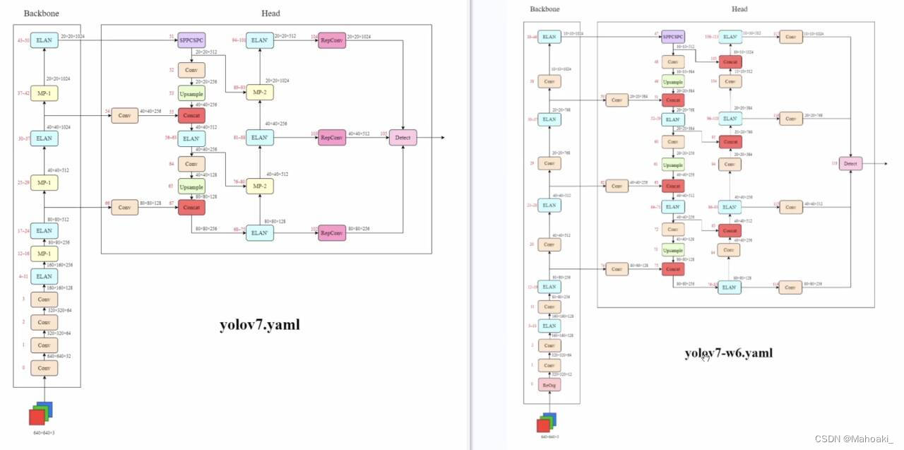
2、backbone和neck部分：

加辅助头的模型有四层输出，路径会更长，粗略看一下：
在这里插入图片描述图源：截图太糊了T^T，可以看一下p3网络结构详解

上图画的是deploy时的w6脚本，没有辅助头。但training和deploy时的backbone以及neck是相同的。

3、head部分：

带辅助头的模型最后一层是IAuxDetect，需要8层的输入，常规的yolov7只有3层输入。

图源：https://arxiv.org/abs/2207.02696

而且w6模型把RepConv都改成了一次3*3的普通卷积：

   # training/yolov7-w6 head
   [83, 1, Conv, [256, 3, 1]],
   [93, 1, Conv, [512, 3, 1]],
   [103, 1, Conv, [768, 3, 1]],
   [113, 1, Conv, [1024, 3, 1]],
   
   [83, 1, Conv, [320, 3, 1]],
   [71, 1, Conv, [640, 3, 1]],
   [59, 1, Conv, [960, 3, 1]],
   [47, 1, Conv, [1280, 3, 1]],

   [[114,115,116,117,118,119,120,121], 1, IAuxDetect, [nc, anchors]],   # Detect(P3, P4, P5, P6)

   # training/yolov7.yaml head
   [75, 1, RepConv, [256, 3, 1]],
   [88, 1, RepConv, [512, 3, 1]],
   [101, 1, RepConv, [1024, 3, 1]],

   [[102,103,104], 1, IDetect, [nc, anchors]],   # Detect(P3, P4, P5)

二、损失计算

这里主要写一下ComputeLossAuxOTA()和ComputeLossOTA()的区别。

1、正样本匹配

折叠一下可以很明了地看到，ComputeLossAuxOTA()多了一个build_targets2()和find_5_positive()。正样本匹配具体内容写过一篇笔记：正样本匹配，现只写辅助头的不同。

在ComputeLossAuxOTA()中可以看到

    def __call__(self, p, targets, imgs):  # predictions, targets, model   
        device = targets.device
        lcls, lbox, lobj = torch.zeros(1, device=device), torch.zeros(1, device=device), torch.zeros(1, device=device)
        bs_aux, as_aux_, gjs_aux, gis_aux, targets_aux, anchors_aux = self.build_targets2(p[:self.nl], targets, imgs)
        bs, as_, gjs, gis, targets, anchors = self.build_targets(p[:self.nl], targets, imgs)

主头和辅助头分别通过build_targets()和build_targets2()选取自己的正样本，而它们传入的参数是相同的，都使用主头的预测值来匹配正样本，辅助头的预测值只用于损失计算。

而build_targets()和build_targets2()的区别也只有最开始的一行代码：使用find_3_positive()还是find_5_positive()，二者区别如下：
在这里插入图片描述图源：https://arxiv.org/abs/2207.02696

正样本匹配第二步时，辅助头选取相邻的4个格子，共5个格子，对比主头3个，正样本更多，可以提高召回率。

2、损失函数

加辅助头的损失函数需要额外加上0.25倍辅助头的损失：

lbox += (1.0 - iou).mean()  # iou loss
lbox += 0.25 * (1.0 - iou_aux).mean()  # iou loss

lcls += self.BCEcls(ps[:, 5:], t)  # BCE
lcls += 0.25 * self.BCEcls(ps_aux[:, 5:], t_aux)  # BCE

obji = self.BCEobj(pi[..., 4], tobj)
obji_aux = self.BCEobj(pi_aux[..., 4], tobj_aux)
lobj += obji * self.balance[i] + 0.25 * obji_aux * self.balance[i]  # obj loss

辅助头计算iou_aux、obji_aux，以及提取ps_aux用的预测值都是辅助头自己的输出，辅助头和主头损失计算方法相同，各算各的。

附：损失函数

具体损失函数计算，以常规的yolov7为例，位置损失和分类损失都只计算正样本计算损失，置信度损失正负样本都要计算：

（1）回归损失（位置损失）

代码中使用的是CIOU损失，见bbox_iou()函数内。

IoU、GIoU、DIoU、CIoU、EIoU 5大评价指标

# Regression
grid = torch.stack([gi, gj], dim=1)
pxy = ps[:, :2].sigmoid() * 2. - 0.5
# pxy = ps[:, :2].sigmoid() * 3. - 1.
pwh = (ps[:, 2:4].sigmoid() * 2) ** 2 * anchors[i]
pbox = torch.cat((pxy, pwh), 1)  # predicted box
selected_tbox = targets[i][:, 2:6] * pre_gen_gains[i]
selected_tbox[:, :2] -= grid
iou = bbox_iou(pbox.T, selected_tbox, x1y1x2y2=False, CIoU=True)  # iou(prediction, target)
lbox += (1.0 - iou).mean()  # iou loss

（2）分类损失

真值为one-hot向量，与预测值计算BEC二分类交叉熵损失： $loss=-\frac{1}{N}\sum_{i=1}^{N}[y_i\cdot \log{p_i}+(1-y_i)\cdot\log{(1-p_i)}]$

# Classification
selected_tcls = targets[i][:, 1].long()
if self.nc > 1:  # cls loss (only if multiple classes)
	t = torch.full_like(ps[:, 5:], self.cn, device=device)  # targets
	t[range(n), selected_tcls] = self.cp
    lcls += self.BCEcls(ps[:, 5:], t)  # BCE

（3）置信度损失

置信度真值取1还是IOU，在train.py中定义了一个系数gr：

model.gr = 1.0  # iou loss ratio (obj_loss = 1.0 or iou)

置信度真值：

tobj[b, a, gj, gi] = (1.0 - self.gr) + self.gr * iou.detach().clamp(0).type(tobj.dtype)  # iou ratio

所以代码中选用的是IOU作为真值，所有正样本置信度真值为与其对应真值框的CIOU，负样本真值为0。然后与预测值计算BEC损失：

obji = self.BCEobj(pi[..., 4], tobj)  # 注意这里用的是pi，而不是ps
lobj += obji * self.balance[i]  # obj loss

其中self.balance参数，可以认为是每个特征层的权重：

self.balance = {3: [4.0, 1.0, 0.4]}.get(det.nl, [4.0, 1.0, 0.25, 0.06, .02])

一般取[4.0, 1.0, 0.4]，对应80*80，40*40，20*20三层，提高了对细粒度特征的惩罚力度。

（4）总损失

需要明确一点，这个ComputeLossOTA中计算的损失是一个批次（16张图片）的总损失，正样本匹配生成的也是把16张图片混在一起“正样本索引”（第一个参数就是图片编号），不是一张一张独立的图片分别计算。

lbox *= self.hyp['box']
lobj *= self.hyp['obj']
lcls *= self.hyp['cls']
bs = tobj.shape[0]  # batch size

loss = lbox + lobj + lcls
return loss * bs, torch.cat((lbox, lobj, lcls, loss)).detach()

总损失就是三项损失分别乘以一个超参数再相加。

最后，放一下ComputeLossAuxOTA中的损失函数计算部分的完整代码：

def __call__(self, p, targets, imgs):  # predictions, targets, model   
    device = targets.device
    lcls, lbox, lobj = torch.zeros(1, device=device), torch.zeros(1, device=device), torch.zeros(1, device=device)
    bs_aux, as_aux_, gjs_aux, gis_aux, targets_aux, anchors_aux = self.build_targets2(p[:self.nl], targets, imgs)
    bs, as_, gjs, gis, targets, anchors = self.build_targets(p[:self.nl], targets, imgs)
    pre_gen_gains_aux = [torch.tensor(pp.shape, device=device)[[3, 2, 3, 2]] for pp in p[:self.nl]]
    pre_gen_gains = [torch.tensor(pp.shape, device=device)[[3, 2, 3, 2]] for pp in p[:self.nl]]

    # Losses
    for i in range(self.nl):  # layer index, layer predictions
        pi = p[i]
        pi_aux = p[i + self.nl]
        b, a, gj, gi = bs[i], as_[i], gjs[i], gis[i]  # image, anchor, gridy, gridx
        b_aux, a_aux, gj_aux, gi_aux = bs_aux[i], as_aux_[i], gjs_aux[i], gis_aux[i]  # image, anchor, gridy, gridx
        tobj = torch.zeros_like(pi[..., 0], device=device)  # target obj
        tobj_aux = torch.zeros_like(pi_aux[..., 0], device=device)  # target obj

        n = b.shape[0]  # number of targets
        if n:
            ps = pi[b, a, gj, gi]  # prediction subset corresponding to targets

            # Regression
            grid = torch.stack([gi, gj], dim=1)
            pxy = ps[:, :2].sigmoid() * 2. - 0.5
            pwh = (ps[:, 2:4].sigmoid() * 2) ** 2 * anchors[i]
            pbox = torch.cat((pxy, pwh), 1)  # predicted box
            selected_tbox = targets[i][:, 2:6] * pre_gen_gains[i]
            selected_tbox[:, :2] -= grid
            iou = bbox_iou(pbox.T, selected_tbox, x1y1x2y2=False, CIoU=True)  # iou(prediction, target)
            lbox += (1.0 - iou).mean()  # iou loss

            # Objectness
            tobj[b, a, gj, gi] = (1.0 - self.gr) + self.gr * iou.detach().clamp(0).type(tobj.dtype)  # iou ratio

            # Classification
            selected_tcls = targets[i][:, 1].long()
            if self.nc > 1:  # cls loss (only if multiple classes)
                t = torch.full_like(ps[:, 5:], self.cn, device=device)  # targets
                t[range(n), selected_tcls] = self.cp
                lcls += self.BCEcls(ps[:, 5:], t)  # BCE

            # Append targets to text file
            # with open('targets.txt', 'a') as file:
            #     [file.write('%11.5g ' * 4 % tuple(x) + '\n') for x in torch.cat((txy[i], twh[i]), 1)]

        n_aux = b_aux.shape[0]  # number of targets
        if n_aux:
            ps_aux = pi_aux[b_aux, a_aux, gj_aux, gi_aux]  # prediction subset corresponding to targets
            grid_aux = torch.stack([gi_aux, gj_aux], dim=1)
            pxy_aux = ps_aux[:, :2].sigmoid() * 2. - 0.5
            # pxy_aux = ps_aux[:, :2].sigmoid() * 3. - 1.
            pwh_aux = (ps_aux[:, 2:4].sigmoid() * 2) ** 2 * anchors_aux[i]
            pbox_aux = torch.cat((pxy_aux, pwh_aux), 1)  # predicted box
            selected_tbox_aux = targets_aux[i][:, 2:6] * pre_gen_gains_aux[i]
            selected_tbox_aux[:, :2] -= grid_aux
            iou_aux = bbox_iou(pbox_aux.T, selected_tbox_aux, x1y1x2y2=False, CIoU=True)  # iou(prediction, target)
            lbox += 0.25 * (1.0 - iou_aux).mean()  # iou loss

            # Objectness
            tobj_aux[b_aux, a_aux, gj_aux, gi_aux] = (1.0 - self.gr) + self.gr * iou_aux.detach().clamp(0).type(
                tobj_aux.dtype)  # iou ratio

            # Classification
            selected_tcls_aux = targets_aux[i][:, 1].long()
            if self.nc > 1:  # cls loss (only if multiple classes)
                t_aux = torch.full_like(ps_aux[:, 5:], self.cn, device=device)  # targets
                t_aux[range(n_aux), selected_tcls_aux] = self.cp
                lcls += 0.25 * self.BCEcls(ps_aux[:, 5:], t_aux)  # BCE

        obji = self.BCEobj(pi[..., 4], tobj)
        obji_aux = self.BCEobj(pi_aux[..., 4], tobj_aux)
        lobj += obji * self.balance[i] + 0.25 * obji_aux * self.balance[i]  # obj loss
        if self.autobalance:
            self.balance[i] = self.balance[i] * 0.9999 + 0.0001 / obji.detach().item()

    if self.autobalance:
        self.balance = [x / self.balance[self.ssi] for x in self.balance]
    lbox *= self.hyp['box']
    lobj *= self.hyp['obj']
    lcls *= self.hyp['cls']
    bs = tobj.shape[0]  # batch size

    loss = lbox + lobj + lcls
    return loss * bs, torch.cat((lbox, lobj, lcls, loss)).detach()