


卷积神经网络(Convolutional Neural Network,CNN)
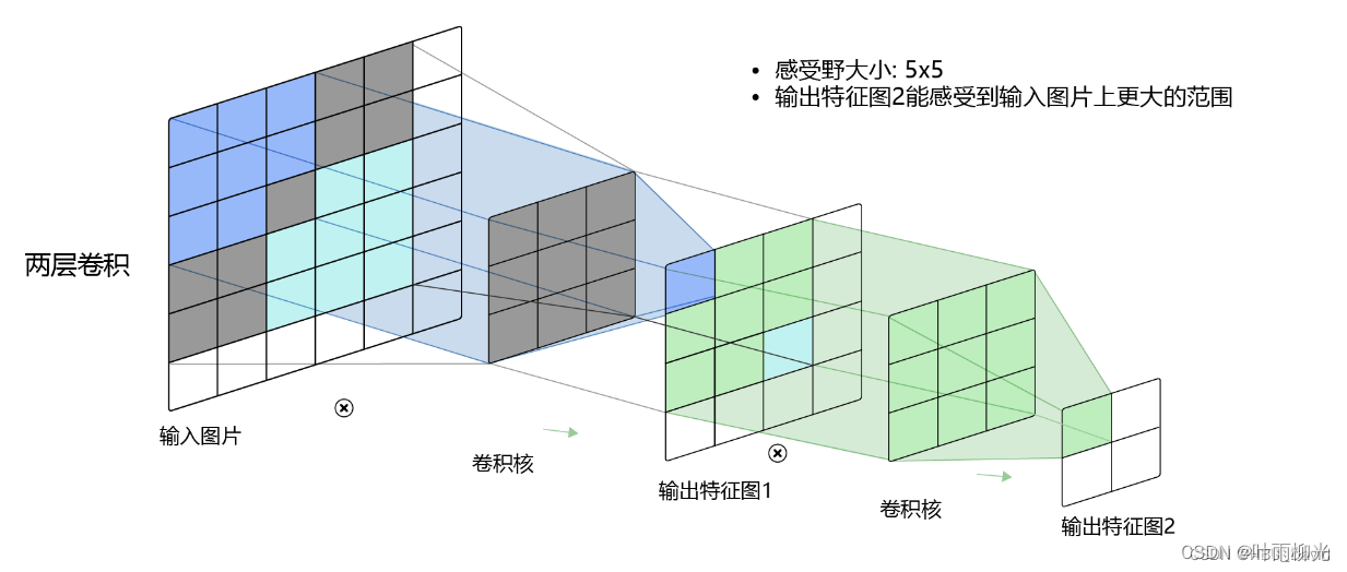
受生物学上感受野机制的启发而提出。
一般是由卷积层、汇聚层和全连接层交叉堆叠而成的前馈神经网络
有三个结构上的特性:局部连接、权重共享、汇聚。
具有一定程度上的平移、缩放和旋转不变性。
和前馈神经网络相比,卷积神经网络的参数更少。
主要应用在图像和视频分析的任务上,其准确率一般也远远超出了其他的神经网络模型。
近年来卷积神经网络也广泛地应用到自然语言处理、推荐系统等领域。
5.1 卷积
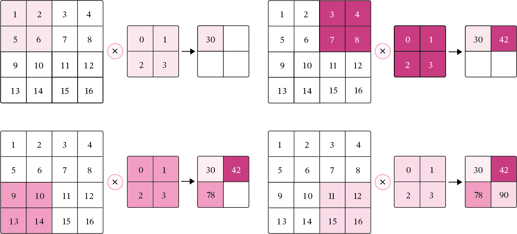
5.1.1 二维卷积运算
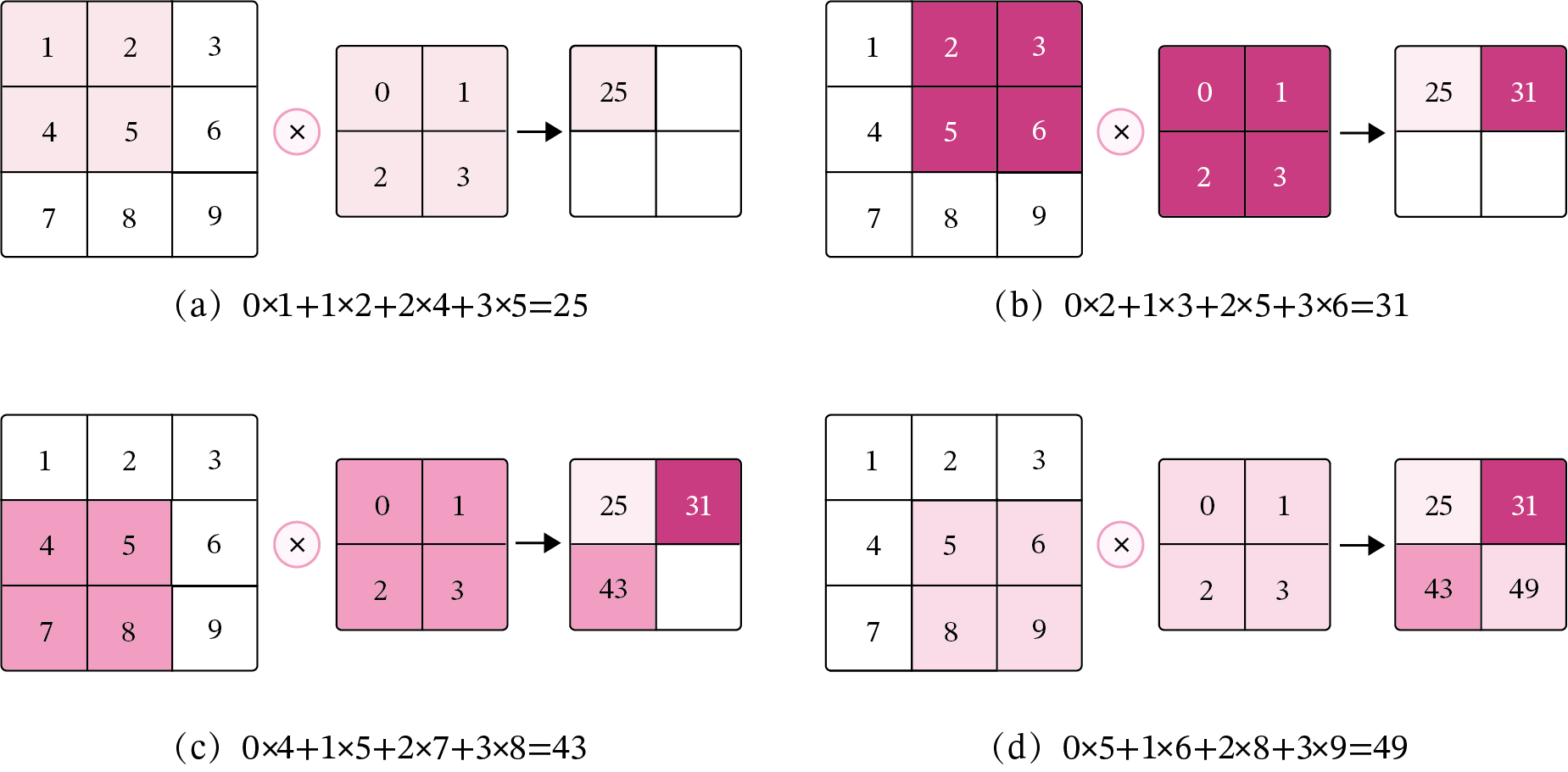
5.1.2 二维卷积算子
在本书后面的实现中,算子都继承paddle.nn.Layer,并使用支持反向传播的飞桨API进行实现,这样我们就可以不用手工写backword()的代码实现。
【使用pytorch实现自定义二维卷积算子】
参考代码:
import torch
import torch.nn as nn
class Conv2D(nn.Module):
def __init__(self, kernel_size,
weight_attr = nn.Parameter(torch.FloatTensor([[0., 1.],[2., 3.]]))):
super(Conv2D, self).__init__()
self.weight = weight_attr
def forward(self, X):
"""
输入:
- X:输入矩阵,shape=[B, M, N],B为样本数量
输出:
- output:输出矩阵
"""
u, v = self.weight.shape
output = torch.zeros([X.shape[0], X.shape[1] - u + 1, X.shape[2] - v + 1])
for i in range(output.shape[1]):
for j in range(output.shape[2]):
output[:, i, j] = torch.sum(X[:, i:i+u, j:j+v]*self.weight, axis=[1,2])
return output
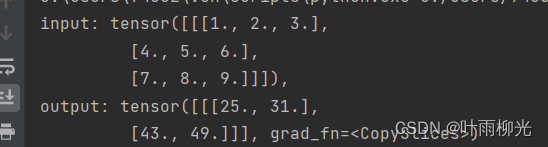
# 随机构造一个二维输入矩阵
inputs = torch.as_tensor([[[1.,2.,3.],[4.,5.,6.],[7.,8.,9.]]])
conv2d = Conv2D(kernel_size=2)
outputs = conv2d(inputs)
print("input: {}, \noutput: {}".format(inputs, outputs))
5.1.3 二维卷积的参数量和计算量
随着隐藏层神经元数量的变多以及层数的加深,
使用全连接前馈网络处理图像数据时,参数量会急剧增加。
如果使用卷积进行图像处理,相较于全连接前馈网络,参数量少了非常多。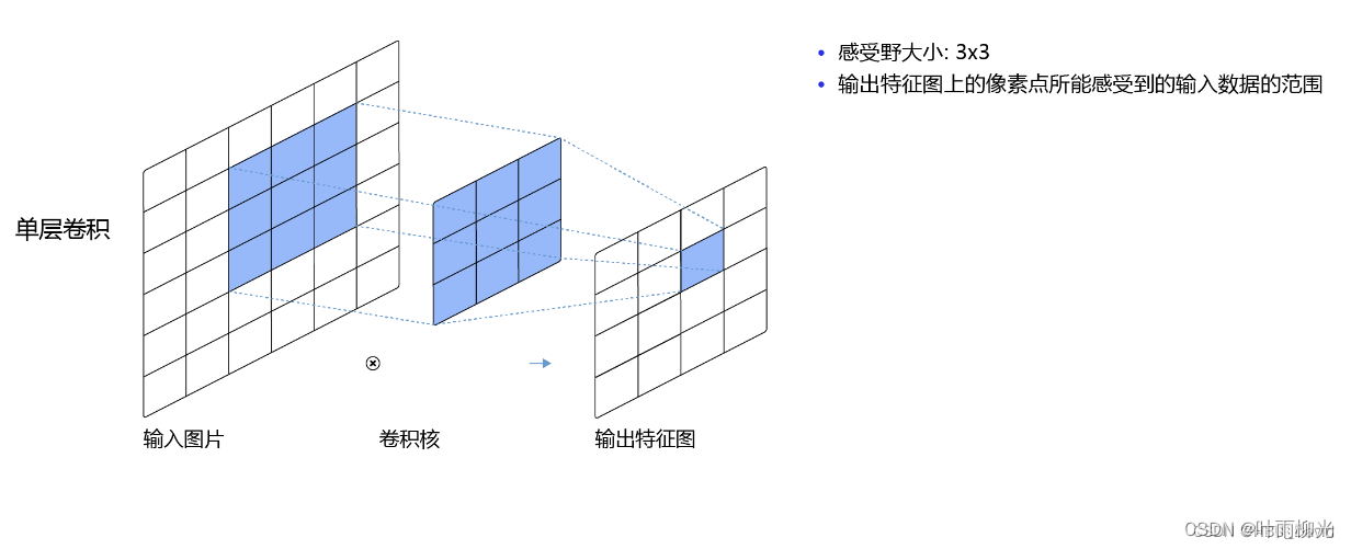
5.1.5 卷积的变种
5.1.5.1 步长(Stride)
5.1.5.2 零填充(Zero Padding)
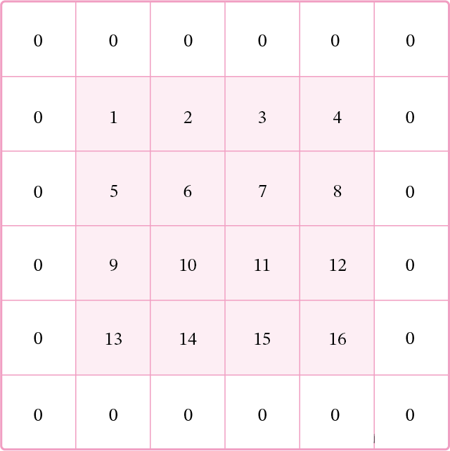
5.1.6 带步长和零填充的二维卷积算子
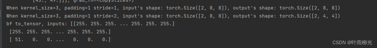
从输出结果看出,使用3×3大小卷积,
padding为1,
当stride=1时,模型的输出特征图与输入特征图保持一致;
当stride=2时,模型的输出特征图的宽和高都缩小一倍。
【使用pytorch实现自定义带步长和零填充的二维卷积算子】
参考代码
class Conv2D(nn.Module):
    def __init__(self, kernel_size, stride=1, padding=0,weight_attr = torch.ones([3,3])):
        super(Conv2D, self).__init__()
        self.weight = weight_attr
        self.weight = self.weight.reshape([kernel_size,kernel_size])
        self.weight = torch.nn.Parameter(weight_attr)
        # 步长
        self.stride = stride
        # 零填充
        self.padding = padding

    def forward(self, X):
        # 零填充
        new_X = torch.zeros([X.shape[0], X.shape[1]+2*self.padding, X.shape[2]+2*self.padding])
        new_X[:, self.padding:X.shape[1]+self.padding, self.padding:X.shape[2]+self.padding] = X
        u, v = self.weight.shape
        output_w = (new_X.shape[1] - u) // self.stride + 1
        output_h = (new_X.shape[2] - v) // self.stride + 1
        output = torch.zeros([X.shape[0], output_w, output_h])
        for i in range(0, output.shape[1]):
            for j in range(0, output.shape[2]):
                output[:, i, j] = torch.sum(
                    new_X[:, self.stride*i:self.stride*i+u, self.stride*j:self.stride*j+v]*self.weight,
                    axis=[1,2])
        return output

inputs = torch.randn(size=[2, 8, 8])
conv2d_padding = Conv2D(kernel_size=3, padding=1)
outputs = conv2d_padding(inputs)
print("When kernel_size=3, padding=1 stride=1, input's shape: {}, output's shape: {}".format(inputs.shape, outputs.shape))
conv2d_stride = Conv2D(kernel_size=3, stride=2, padding=1)
outputs = conv2d_stride(inputs)
print("When kernel_size=3, padding=1 stride=2, input's shape: {}, output's shape: {}".format(inputs.shape, outputs.shape))
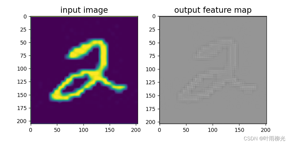
5.1.7 使用卷积运算完成图像边缘检测任务
【使用pytorch实现图像边缘检测】

参考代码
# %matplotlib inline
import matplotlib.pyplot as plt
from PIL import Image
import numpy as np

# 读取图片
img = Image.open('2.png').convert('L')
img.resize((256,256))
# 设置卷积核参数
w = np.array([[-1,-1,-1], [-1,8,-1], [-1,-1,-1]], dtype='float32')
# 创建卷积算子,卷积核大小为3x3,并使用上面的设置好的数值作为卷积核权重的初始化参数
conv = Conv2D(kernel_size=3, stride=1, padding=0, weight_attr=torch.tensor(w))

# 将读入的图片转化为float32类型的numpy.ndarray
inputs = np.array(img).astype('float32')
print("bf to_tensor, inputs:",inputs)
# 将图片转为Tensor
inputs = torch.tensor(inputs)
print("bf unsqueeze, inputs:",inputs)
inputs = torch.unsqueeze(inputs, axis=0)
print("af unsqueeze, inputs:",inputs)
outputs = conv(inputs)
# outputs = outputs.detach().numpy()
# 可视化结果
plt.figure(figsize=(8, 4))
f = plt.subplot(121)
f.set_title('input image', fontsize=15)
plt.imshow(img)
f = plt.subplot(122)
f.set_title('output feature map', fontsize=15)
plt.imshow(outputs.detach().numpy().squeeze(), cmap='gray')
plt.savefig('conv-vis.pdf')
plt.show()
选做题
1.实现一些传统边缘检测算子,如:Roberts、Prewitt、Sobel、Scharr、Kirsch、Robinson、Laplacia```python
import cv2
import numpy as np
# 加载图像
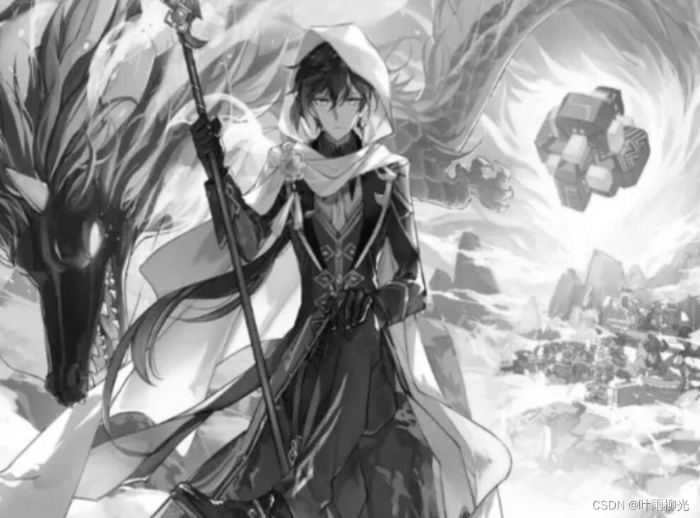
image = cv2.imread('zhongli.png', 0)
image = cv2.resize(image, (800, 800))
# 自定义卷积核
# Roberts边缘算子
kernel_Roberts_x = np.array([
[1, 0],
[0, -1]
])
kernel_Roberts_y = np.array([
[0, -1],
[1, 0]
])
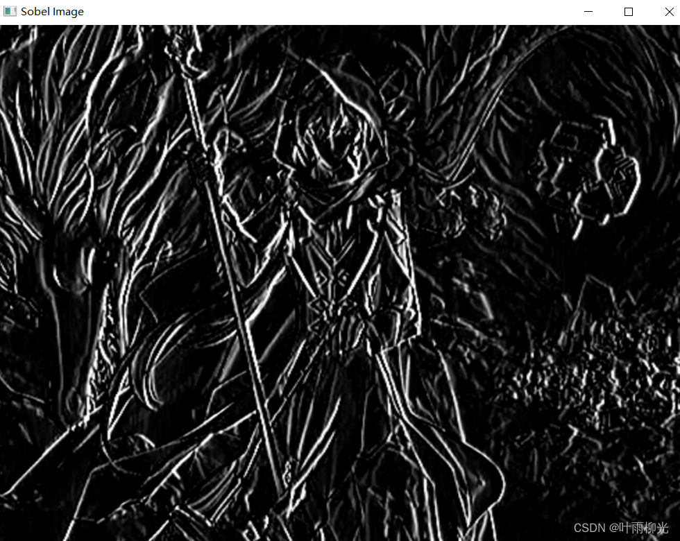
# Sobel边缘算子
kernel_Sobel_x = np.array([
[-1, 0, 1],
[-2, 0, 2],
[-1, 0, 1]])
kernel_Sobel_y = np.array([
[1, 2, 1],
[0, 0, 0],
[-1, -2, -1]])
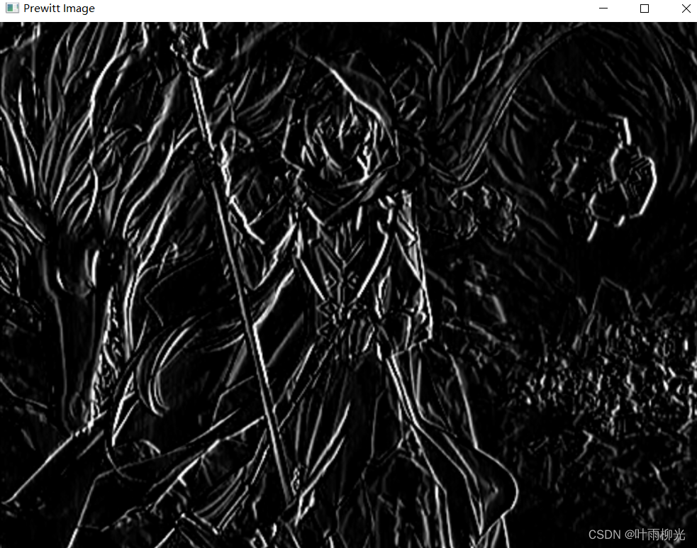
# Prewitt边缘算子
kernel_Prewitt_x = np.array([
[-1, 0, 1],
[-1, 0, 1],
[-1, 0, 1]])
kernel_Prewitt_y = np.array([
[1, 1, 1],
[0, 0, 0],
[-1, -1, -1]])
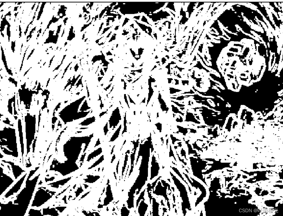
# Kirsch 边缘检测算子
def kirsch(image):
m, n = image.shape
list = []
kirsch = np.zeros((m, n))
for i in range(2, m - 1):
for j in range(2, n - 1):
d1 = np.square(5 * image[i - 1, j - 1] + 5 * image[i - 1, j] + 5 * image[i - 1, j + 1] -
3 * image[i, j - 1] - 3 * image[i, j + 1] - 3 * image[i + 1, j - 1] -
3 * image[i + 1, j] - 3 * image[i + 1, j + 1])
d2 = np.square((-3) * image[i - 1, j - 1] + 5 * image[i - 1, j] + 5 * image[i - 1, j + 1] -
3 * image[i, j - 1] + 5 * image[i, j + 1] - 3 * image[i + 1, j - 1] -
3 * image[i + 1, j] - 3 * image[i + 1, j + 1])
d3 = np.square((-3) * image[i - 1, j - 1] - 3 * image[i - 1, j] + 5 * image[i - 1, j + 1] -
3 * image[i, j - 1] + 5 * image[i, j + 1] - 3 * image[i + 1, j - 1] -
3 * image[i + 1, j] + 5 * image[i + 1, j + 1])
d4 = np.square((-3) * image[i - 1, j - 1] - 3 * image[i - 1, j] - 3 * image[i - 1, j + 1] -
3 * image[i, j - 1] + 5 * image[i, j + 1] - 3 * image[i + 1, j - 1] +
5 * image[i + 1, j] + 5 * image[i + 1, j + 1])
d5 = np.square((-3) * image[i - 1, j - 1] - 3 * image[i - 1, j] - 3 * image[i - 1, j + 1] - 3
* image[i, j - 1] - 3 * image[i, j + 1] + 5 * image[i + 1, j - 1] +
5 * image[i + 1, j] + 5 * image[i + 1, j + 1])
d6 = np.square((-3) * image[i - 1, j - 1] - 3 * image[i - 1, j] - 3 * image[i - 1, j + 1] +
5 * image[i, j - 1] - 3 * image[i, j + 1] + 5 * image[i + 1, j - 1] +
5 * image[i + 1, j] - 3 * image[i + 1, j + 1])
d7 = np.square(5 * image[i - 1, j - 1] - 3 * image[i - 1, j] - 3 * image[i - 1, j + 1] +
5 * image[i, j - 1] - 3 * image[i, j + 1] + 5 * image[i + 1, j - 1] -
3 * image[i + 1, j] - 3 * image[i + 1, j + 1])
d8 = np.square(5 * image[i - 1, j - 1] + 5 * image[i - 1, j] - 3 * image[i - 1, j + 1] +
5 * image[i, j - 1] - 3 * image[i, j + 1] - 3 * image[i + 1, j - 1] -
3 * image[i + 1, j] - 3 * image[i + 1, j + 1])
# 第一种方法:取各个方向的最大值,效果并不好,采用另一种方法
list = [d1, d2, d3, d4, d5, d6, d7, d8]
kirsch[i, j] = int(np.sqrt(max(list)))
for i in range(m):
for j in range(n):
if kirsch[i, j] > 127:
kirsch[i, j] = 255
else:
kirsch[i, j] = 0
return kirsch
# 拉普拉斯卷积核
kernel_Laplacian_1 = np.array([
[0, 1, 0],
[1, -4, 1],
[0, 1, 0]])
kernel_Laplacian_2 = np.array([
[1, 1, 1],
[1, -8, 1],
[1, 1, 1]])
# 下面两个卷积核不具有旋转不变性
kernel_Laplacian_3 = np.array([
[2, -1, 2],
[-1, -4, -1],
[2, 1, 2]])
kernel_Laplacian_4 = np.array([
[-1, 2, -1],
[2, -4, 2],
[-1, 2, -1]])
# 5*5 LoG卷积模板
kernel_LoG = np.array([
[0, 0, -1, 0, 0],
[0, -1, -2, -1, 0],
[-1, -2, 16, -2, -1],
[0, -1, -2, -1, 0],
[0, 0, -1, 0, 0]])
# 卷积
output_1 = cv2.filter2D(image, -1, kernel_Prewitt_x)
output_2 = cv2.filter2D(image, -1, kernel_Sobel_x)
output_3 = cv2.filter2D(image, -1, kernel_Prewitt_x)
output_4 = cv2.filter2D(image, -1, kernel_Laplacian_1)
output_5 = kirsch(image)
# 显示锐化效果
image = cv2.resize(image, (800, 600))
output_1 = cv2.resize(output_1, (800, 600))
output_2 = cv2.resize(output_2, (800, 600))
output_3 = cv2.resize(output_3, (800, 600))
output_4 = cv2.resize(output_4, (800, 600))
output_5 = cv2.resize(output_5, (800, 600))
cv2.imshow('Original Image', image)
cv2.imshow('Prewitt Image', output_1)
cv2.imshow('Sobel Image', output_2)
cv2.imshow('Prewitt Image', output_3)
cv2.imshow('Laplacian Image', output_4)
cv2.imshow('kirsch Image', output_5)
# 停顿
if cv2.waitKey(0) & 0xFF == 27:
cv2.destroyAllWindows()

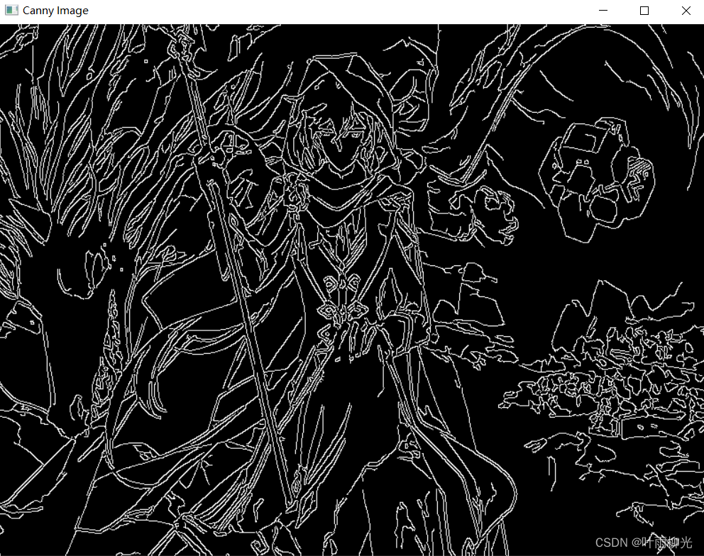
2.实现的简易的 Canny 边缘检测算法
import cv2
# 加载图像
image = cv2.imread('lu.png',0)
image = cv2.resize(image,(800,800))
def Canny(image,k,t1,t2):
    img = cv2.GaussianBlur(image, (k, k), 0)
    canny = cv2.Canny(img, t1, t2)
    return canny
image = cv2.resize(image, (800, 600))
cv2.imshow('Original Image', image)
output =cv2.resize(Canny(image,3,50,150),(800,600))
cv2.imshow('Canny Image', output)
# 停顿
if cv2.waitKey(0) & 0xFF == 27:
    cv2.destroyAllWindows()
总结
因为上节课做过卷积作业,所以本次实验并不是那么难,主要是观察一下带步长、不带步长和带填充、不带填充的效果以及使用卷积算子做边缘检测任务。


 1万+
1万+


 被折叠的 条评论
为什么被折叠?
被折叠的 条评论
为什么被折叠?
 到【灌水乐园】发言


