Transformer时间序列预测：多变量输入与多变量输出

引言

任务描述

使用100个时间步的多变量时间序列预测未来20个时间步的目标序列。自变量有10个，因变量也有10个。

代码参考：

https://github.com/oliverguhr/transformer-time-series-prediction

https://github.com/RuifMaxx/Multidimensional-time-series-with-transformer

数据集描述：

https://archive.ics.uci.edu/dataset/321/electricityloaddiagrams20112014

数据集下载：

https://drive.google.com/file/d/13FyJqP_MVVHzqQ3G0egpglelO0G-dsEa/view

运行配置

以下代码在GPU上运行成功。

import torch
import torch.nn as nn
from torch.utils.data import DataLoader, TensorDataset
import numpy as np
import random
import math
from sklearn.preprocessing import MinMaxScaler
import pandas as pd
from datetime import date
import time
import matplotlib.pyplot as plt
from matplotlib_inline import backend_inline 
backend_inline.set_matplotlib_formats('svg')
 
input_window = 100
output_window = 20 # 预测一段时间序列未来 20 个时间步的值
batch_size = 32 
device = torch.device("cuda" if torch.cuda.is_available() else "cpu")

位置编码

class PositionalEncoding(nn.Module):
    
    def __init__(self, d_model, max_len=5000):
        super(PositionalEncoding, self).__init__()       
        pe = torch.zeros(max_len, d_model)
        position = torch.arange(0, max_len, dtype=torch.float).unsqueeze(1)
        div_term = torch.exp(torch.arange(0, d_model, 2).float() * (-math.log(10000.0) / d_model))
        pe[:, 0::2] = torch.sin(position * div_term)
        pe[:, 1::2] = torch.cos(position * div_term)
        pe = pe.unsqueeze(0).transpose(0, 1)
        self.register_buffer('pe', pe)

    def forward(self, x):
        return x + self.pe[:x.size(0), :] # [input_window, batch size, embed dim]

transformer

这里的解码器用一个全连接层表示，然后再加一个全连接层得到最后输出。

class TransAm(nn.Module):
    def __init__(self, series_dim, feature_size = 80, num_layers=3, dropout=0.5):
        super(TransAm, self).__init__()
        self.model_type = 'Transformer'
        self.src_mask = None
        self.input_embedding = nn.Linear(series_dim, feature_size)
        self.pos_encoder = PositionalEncoding(feature_size)
        self.encoder_layer = nn.TransformerEncoderLayer(d_model=feature_size, nhead=10, dropout=dropout)
        self.transformer_encoder = nn.TransformerEncoder(self.encoder_layer, num_layers=num_layers)        
        self.decoder = nn.Linear(feature_size, feature_size//2)
        self.out = nn.Linear(feature_size//2, series_dim)
        self.init_weights()

    def init_weights(self):
        initrange = 0.1    
        self.decoder.bias.data.zero_()
        # 将解码器的权重初始化为均匀分布的随机值，范围在 [−0.1,0.1] 之间
        self.decoder.weight.data.uniform_(-initrange, initrange)

    def forward(self,src):
        if self.src_mask is None or self.src_mask.size(0) != len(src):
            device = src.device
            mask = self._generate_square_subsequent_mask(len(src)).to(device)
            self.src_mask = mask
        src = self.input_embedding(src)
        src = self.pos_encoder(src) # [input_window, batch_size, feature_size]
        en_output = self.transformer_encoder(src, self.src_mask) 
        de_output = self.decoder(en_output) # [input_window, batch_size, feature_size//2]
        out_put = self.out(de_output[-output_window:,:,:])
        return out_put # [output_window, batch_size, series_dim]

    def _generate_square_subsequent_mask(self, sz):
        '''
        生成一个上三角掩码矩阵，防止模型在预测时看到未来时间步的数据。若 sz = 4 则生成：
        [[0.0,   -inf,  -inf,  -inf],
        [0.0,    0.0,  -inf,  -inf],
        [0.0,    0.0,   0.0,  -inf],
        [0.0,    0.0,   0.0,   0.0]]
        '''
        mask = (torch.triu(torch.ones(sz, sz)) == 1).transpose(0, 1)
        mask = mask.float().masked_fill(mask == 0, float('-inf')).masked_fill(mask == 1, float(0.0))
        return mask

创建特征和标签

data_ = pd.read_csv('/kaggle/input/ld-20142/LD_20142.csv', parse_dates=["date"])
data_.head()

	date	time	time24	MT_001	MT_002	MT_003	MT_004	MT_005	MT_006	MT_007	...	MT_361	MT_362	MT_363	MT_364	MT_365	MT_366	MT_367	MT_368	MT_369	MT_370
0	2013-12-30	0.593750	14.25	1.269036	29.871977	0.868810	144.308943	64.634146	330.357143	3.957038	...	368.308351	46300	3535.864979	3363.636364	91.264668	9.362200	256.365233	178.631052	824.046921	17135.13514
1	2013-12-30	0.604167	14.50	1.269036	29.160740	1.737619	138.211382	65.853659	300.595238	3.391747	...	379.728765	46200	3573.839662	3454.545455	91.264668	8.191925	246.707638	180.300501	846.774194	17081.08108
2	2013-12-30	0.614583	14.75	1.269036	29.160740	1.737619	154.471545	60.975610	312.500000	3.957038	...	438.258387	46800	3573.839662	3340.909091	95.176010	8.777063	252.853380	183.639399	824.046921	17459.45946
3	2013-12-30	0.625000	15.00	2.538071	28.449502	1.737619	154.471545	57.317073	264.880952	4.522329	...	434.689507	46800	3586.497890	3340.909091	89.960887	12.873025	255.487269	186.978297	821.114369	18702.70270
4	2013-12-30	0.635417	15.25	2.538071	28.449502	0.868810	144.308943	54.878049	279.761905	4.522329	...	412.562455	51700	3573.839662	3545.454545	89.960887	11.702750	253.731343	185.308848	847.507331	19243.24324

5 rows × 373 columns

def create_inout_sequences(input_data, input_window):
    inout_seq = []
    L = len(input_data)
    for i in range(L - input_window - output_window + 1):
        train_seq = input_data[i : i + input_window]
        train_label = input_data[i + input_window : i  + input_window + output_window]
        inout_seq.append((train_seq ,train_label))
    return inout_seq

def get_data():
    # 归一化: 将原始数据中的最小值映射到 -1，最大值映射到 1
    scaler = MinMaxScaler(feature_range=(-1, 1)) 
    data = data_.loc[
        (data_["date"] >= pd.Timestamp(date(2014, 1, 1))) & (data_["date"] <= pd.Timestamp(date(2014, 4, 14)))]
    data = data.loc[:, "MT_200": "MT_209"]
    print('初始时序数据：', data.shape)
    series = data.to_numpy()
    amplitude = scaler.fit_transform(series)
    split = int(0.8 * data.shape[0])
    train_data = amplitude[:split]
    test_data = amplitude[split:]
    print('切分序列为训练数据和测试数据：', train_data.shape, test_data.shape)
    
    train_sequence = create_inout_sequences(train_data, input_window)
    test_data = create_inout_sequences(test_data, input_window)
    
    return train_sequence, test_data, scaler

# 取出一个batch的数据
def get_batch(source, i, batch_size):
    sample_num = min(batch_size, len(source) - i) # 最后一个batch的样本数可能少于batch_size，即 1<=len(source) - i<batch_size
    data = source[i: i + sample_num] # data 即为一个 batch 中的数据，有 sample_num 个样本
    # torch.stack([item[0] for item in data])的形状是(batch_size, input_window, series_dim)
    # .chunk(input_window,1)会将时间步维度的每个序列切分为 input_window 个小张量，每个小张量的形状将是 (batch_size, 1, series_dim)
    # 最外层的torch.stack：再进行一次堆叠，把它们重新组合成一个新的张量，形状为 (input_window, batch_size, 1, series_dim)
    # 最后去掉一个维度，变成(input_window, batch_size, series_dim)
    # 其实就是把将 input_window 和 batch_size 的维度交换
    input = torch.stack(torch.stack([torch.tensor(item[0], dtype=torch.float32) for item in data]).chunk(input_window,1)).squeeze() 
    target = torch.stack(torch.stack([torch.tensor(item[1], dtype=torch.float32) for item in data]).chunk(output_window,1)).squeeze()
    return input.to(device), target.to(device)

train_data, val_data, scaler = get_data()
print('训练样本数量:', len(train_data))
print('测试样本数量:', len(val_data))
tr,te = get_batch(train_data, 0, batch_size)
print('一个batch中的数据形状：', tr.shape, te.shape) 
# 分别为 [input_window, batch_size, series_dim] 和 [output_window, batch_size, series_dim]

初始时序数据： (9896, 10)
切分序列为训练数据和测试数据： (7916, 10) (1980, 10)
训练样本数量: 7797
测试样本数量: 1861
一个batch中的数据形状： torch.Size([100, 32, 10]) torch.Size([20, 32, 10])

train_data是一个列表，元素为元组，元组有两个元素，第一个为特征，第二个为标签。

训练函数

def train(train_data):
    model.train()
    total_loss = 0.
    start_time = time.time()
    indices = list(range(0, len(train_data), batch_size)) 
    random.shuffle(indices)
    for batch, i in enumerate(indices):
        data, targets = get_batch(train_data, i, batch_size)
        optimizer.zero_grad()
        output = model(data) # [output_window, batch_size, series_dim]        
        loss = criterion(output, targets)
        loss.backward()
        # 当调用 clip_grad_norm_ 时，函数会计算所有参数梯度的范数。
        # 如果这个范数超过指定的阈值（0.7），则会将所有梯度缩放，以确保它们的范数不超过 0.7
        torch.nn.utils.clip_grad_norm_(model.parameters(), 0.7)
        optimizer.step()

        total_loss += loss.item()
        log_interval = int(len(train_data) / batch_size / 5)
        # 每经过一定数量的批次就打印一次日志
        if batch % log_interval == 0 and batch > 0:
            elapsed = time.time() - start_time
            print('| epoch {:3d} | {:5d}/{:5d} batches | '
                  'lr {:02.6f} | {:5.2f} ms | '
                  'loss {:5.5f}'.format(
                    epoch, batch, len(train_data) // batch_size, scheduler.get_last_lr()[0],
                    elapsed * 1000,
                    total_loss))
            total_loss = 0
            start_time = time.time()

绘图函数

def plot(eval_model, data_source, epoch, scaler):
    eval_model.eval() 
    total_loss = 0.
    test_result = torch.Tensor(0)    
    truth = torch.Tensor(0)
    with torch.no_grad():
        for i in range(0, len(data_source) - 1):
            data, target = get_batch(data_source, i, 1) # 在预测时是一个一个样本进行预测，即batch_size=1
            # data.shape：[100,10] target.shape：[20,10]
            data = data.unsqueeze(1)
            target = target.unsqueeze(1)            
            output = eval_model(data)
#             print('预测结果形状：',output.shape) # torch.Size([20, 1, 10])                             
            total_loss += criterion(output, target).item()
            
            # 以下代码用于画图
            # output[-output_window,:].shape: torch.Size([1, 10])
            test_result = torch.cat((test_result, output[-output_window,:].cpu()), 0)
            truth = torch.cat((truth, target[-output_window,:].cpu()), 0)
            
    test_result_=scaler.inverse_transform(test_result[:700])
    truth_=scaler.inverse_transform(truth[:700])
#     print(test_result_.shape,test_result_) # (700, 10)
    for m in range(0,1): # 这里只画第一个目标值的时序图
        test_result = test_result_[:,m]
        truth = truth_[:,m]
        print('MAE:', np.mean(np.abs(test_result-truth)))
        print('MSE:', np.mean((test_result-truth)**2))
        fig = plt.figure(1, figsize=(14, 5))
        fig.patch.set_facecolor('xkcd:white')
        plt.plot(test_result[:700],color="red") 
        plt.title('Test Prediction')
        plt.plot(truth[:700],color="black")
        plt.legend(["prediction", "true"], loc="upper left")
        ymin, ymax = plt.ylim()
#         plt.vlines(500, ymin, ymax, color="blue", linestyles="dashed", linewidth=2)
        plt.ylim(ymin, ymax)
        plt.xlabel("Periods")
        plt.ylabel(f"Y{m+1}")
        plt.show()
        plt.close()
    return total_loss # 用来保存最佳模型

训练和预测

train_data, val_data, scaler = get_data()
model = TransAm(series_dim = 10).to(device)

criterion = nn.MSELoss()
lr = 0.001
# optimizer = torch.optim.SGD(model.parameters(), lr=lr)
optimizer = torch.optim.AdamW(model.parameters(), lr=lr) # AdamW 在更新过程中考虑了权重衰减（L2正则化）
# 使用分步学习率调度器，旨在在训练过程中逐渐减小学习率，每隔 1 个 epoch 进行一次学习率更新
# 每次更新时将学习率乘以 gamma（0.9），也就是说，学习率会在每个 epoch 后减少 10%
scheduler = torch.optim.lr_scheduler.StepLR(optimizer, 1.0, gamma=0.9)

best_val_loss = float("inf")
epochs = 10 
best_model = None

for epoch in range(1, epochs + 1):
    epoch_start_time = time.time()
    train(train_data)
    
    if(epoch % 1 == 0):
        val_loss = plot(model, val_data, epoch, scaler)
        
    print('-' * 89)
    print('| end of epoch {:3d} | time: {:5.2f}s | valid loss {:5.5f}'.format(epoch, (time.time() - epoch_start_time),val_loss))
    print('-' * 89)

    if val_loss < best_val_loss:
       best_val_loss = val_loss
       best_model = model

    scheduler.step() 
print('best_val_loss', best_val_loss)
torch.save(model.state_dict(), 'model.pt')

初始时序数据： (9896, 10)
切分序列为训练数据和测试数据： (7916, 10) (1980, 10)


| epoch   1 |    48/  243 batches | lr 0.001000 | 1526.59 ms | loss 7.42650
| epoch   1 |    96/  243 batches | lr 0.001000 | 764.55 ms | loss 5.90667
| epoch   1 |   144/  243 batches | lr 0.001000 | 758.76 ms | loss 6.07634
| epoch   1 |   192/  243 batches | lr 0.001000 | 759.10 ms | loss 5.97583
| epoch   1 |   240/  243 batches | lr 0.001000 | 766.38 ms | loss 4.33366
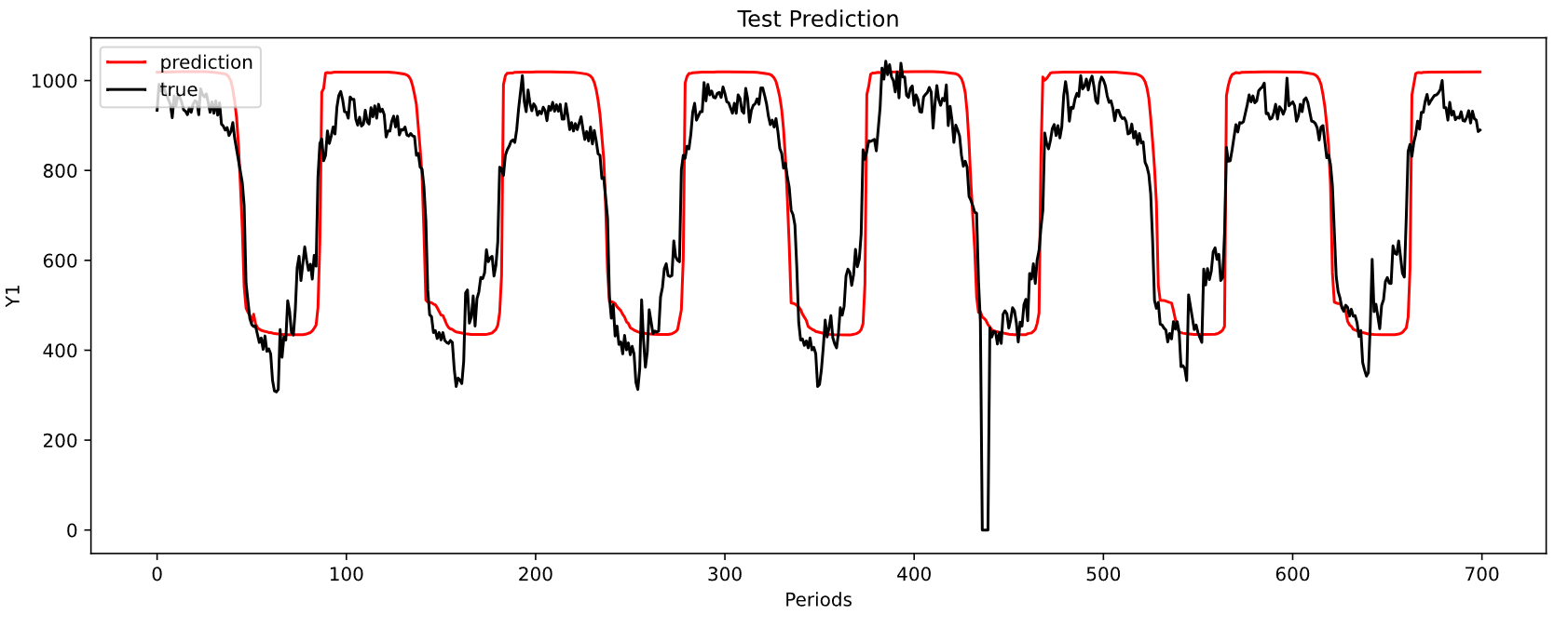
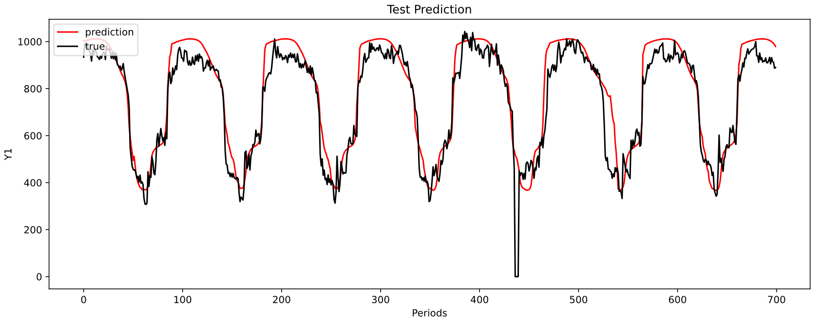
MAE: 90.2560738177567
MSE: 12069.72568232489

-----------------------------------------------------------------------------------------
| end of epoch   1 | time:  9.80s | valid loss 130.09003
-----------------------------------------------------------------------------------------
| epoch   2 |    48/  243 batches | lr 0.000900 | 903.66 ms | loss 1.88771
| epoch   2 |    96/  243 batches | lr 0.000900 | 773.30 ms | loss 1.34669
| epoch   2 |   144/  243 batches | lr 0.000900 | 762.35 ms | loss 1.31896
| epoch   2 |   192/  243 batches | lr 0.000900 | 771.85 ms | loss 1.05898
| epoch   2 |   240/  243 batches | lr 0.000900 | 766.26 ms | loss 1.66898
MAE: 130.74233856178395
MSE: 21928.816309675996

-----------------------------------------------------------------------------------------
| end of epoch   2 | time:  9.16s | valid loss 78.91797
-----------------------------------------------------------------------------------------
| epoch   3 |    48/  243 batches | lr 0.000810 | 895.13 ms | loss 0.89362
| epoch   3 |    96/  243 batches | lr 0.000810 | 765.58 ms | loss 1.10743
| epoch   3 |   144/  243 batches | lr 0.000810 | 770.17 ms | loss 1.02959
| epoch   3 |   192/  243 batches | lr 0.000810 | 756.66 ms | loss 1.08448
| epoch   3 |   240/  243 batches | lr 0.000810 | 775.35 ms | loss 0.83710
MAE: 95.88788747427077
MSE: 14549.661332151985

-----------------------------------------------------------------------------------------
| end of epoch   3 | time:  9.28s | valid loss 57.86707
-----------------------------------------------------------------------------------------
| epoch   4 |    48/  243 batches | lr 0.000729 | 889.70 ms | loss 0.84351
| epoch   4 |    96/  243 batches | lr 0.000729 | 767.70 ms | loss 1.13962
| epoch   4 |   144/  243 batches | lr 0.000729 | 763.74 ms | loss 0.79985
| epoch   4 |   192/  243 batches | lr 0.000729 | 770.92 ms | loss 0.79263
| epoch   4 |   240/  243 batches | lr 0.000729 | 773.83 ms | loss 1.19982
MAE: 76.44456674668267
MSE: 8620.984164154655

-----------------------------------------------------------------------------------------
| end of epoch   4 | time:  9.38s | valid loss 48.19368
-----------------------------------------------------------------------------------------
| epoch   5 |    48/  243 batches | lr 0.000656 | 899.48 ms | loss 0.77779
| epoch   5 |    96/  243 batches | lr 0.000656 | 772.83 ms | loss 0.91519
| epoch   5 |   144/  243 batches | lr 0.000656 | 773.17 ms | loss 0.89872
| epoch   5 |   192/  243 batches | lr 0.000656 | 763.26 ms | loss 0.78820
| epoch   5 |   240/  243 batches | lr 0.000656 | 780.71 ms | loss 0.99669
MAE: 59.14287770249517
MSE: 6958.48955422965

-----------------------------------------------------------------------------------------
| end of epoch   5 | time:  9.24s | valid loss 46.28011
-----------------------------------------------------------------------------------------
| epoch   6 |    48/  243 batches | lr 0.000590 | 895.63 ms | loss 0.89292
| epoch   6 |    96/  243 batches | lr 0.000590 | 778.87 ms | loss 0.79402
| epoch   6 |   144/  243 batches | lr 0.000590 | 782.59 ms | loss 0.69588
| epoch   6 |   192/  243 batches | lr 0.000590 | 777.70 ms | loss 0.98849
| epoch   6 |   240/  243 batches | lr 0.000590 | 776.67 ms | loss 0.73527
MAE: 78.68922871430728
MSE: 9402.826728924343

-----------------------------------------------------------------------------------------
| end of epoch   6 | time:  9.44s | valid loss 51.03970
-----------------------------------------------------------------------------------------
| epoch   7 |    48/  243 batches | lr 0.000531 | 884.70 ms | loss 0.76392
| epoch   7 |    96/  243 batches | lr 0.000531 | 786.16 ms | loss 0.73662
| epoch   7 |   144/  243 batches | lr 0.000531 | 780.03 ms | loss 0.99307
| epoch   7 |   192/  243 batches | lr 0.000531 | 782.99 ms | loss 1.01473
| epoch   7 |   240/  243 batches | lr 0.000531 | 779.67 ms | loss 0.75703
MAE: 79.88809012856592
MSE: 9700.616121160681

-----------------------------------------------------------------------------------------
| end of epoch   7 | time:  9.25s | valid loss 50.65413
-----------------------------------------------------------------------------------------
| epoch   8 |    48/  243 batches | lr 0.000478 | 903.40 ms | loss 0.80129
| epoch   8 |    96/  243 batches | lr 0.000478 | 786.61 ms | loss 0.76111
| epoch   8 |   144/  243 batches | lr 0.000478 | 783.58 ms | loss 0.70030
| epoch   8 |   192/  243 batches | lr 0.000478 | 771.34 ms | loss 0.78637
| epoch   8 |   240/  243 batches | lr 0.000478 | 778.09 ms | loss 0.90822
MAE: 85.46249401894232
MSE: 11243.749225793306

-----------------------------------------------------------------------------------------
| end of epoch   8 | time:  9.20s | valid loss 44.89603
-----------------------------------------------------------------------------------------
| epoch   9 |    48/  243 batches | lr 0.000430 | 887.70 ms | loss 0.77369
| epoch   9 |    96/  243 batches | lr 0.000430 | 786.48 ms | loss 0.74093
| epoch   9 |   144/  243 batches | lr 0.000430 | 779.69 ms | loss 0.74708
| epoch   9 |   192/  243 batches | lr 0.000430 | 777.35 ms | loss 0.75861
| epoch   9 |   240/  243 batches | lr 0.000430 | 779.19 ms | loss 0.83453
MAE: 61.53478251329422
MSE: 7324.079512784931

-----------------------------------------------------------------------------------------
| end of epoch   9 | time:  9.20s | valid loss 43.55069
-----------------------------------------------------------------------------------------
| epoch  10 |    48/  243 batches | lr 0.000387 | 908.86 ms | loss 0.75782
| epoch  10 |    96/  243 batches | lr 0.000387 | 784.92 ms | loss 0.75925
| epoch  10 |   144/  243 batches | lr 0.000387 | 790.59 ms | loss 0.73587
| epoch  10 |   192/  243 batches | lr 0.000387 | 785.02 ms | loss 0.65881
| epoch  10 |   240/  243 batches | lr 0.000387 | 784.74 ms | loss 0.88428
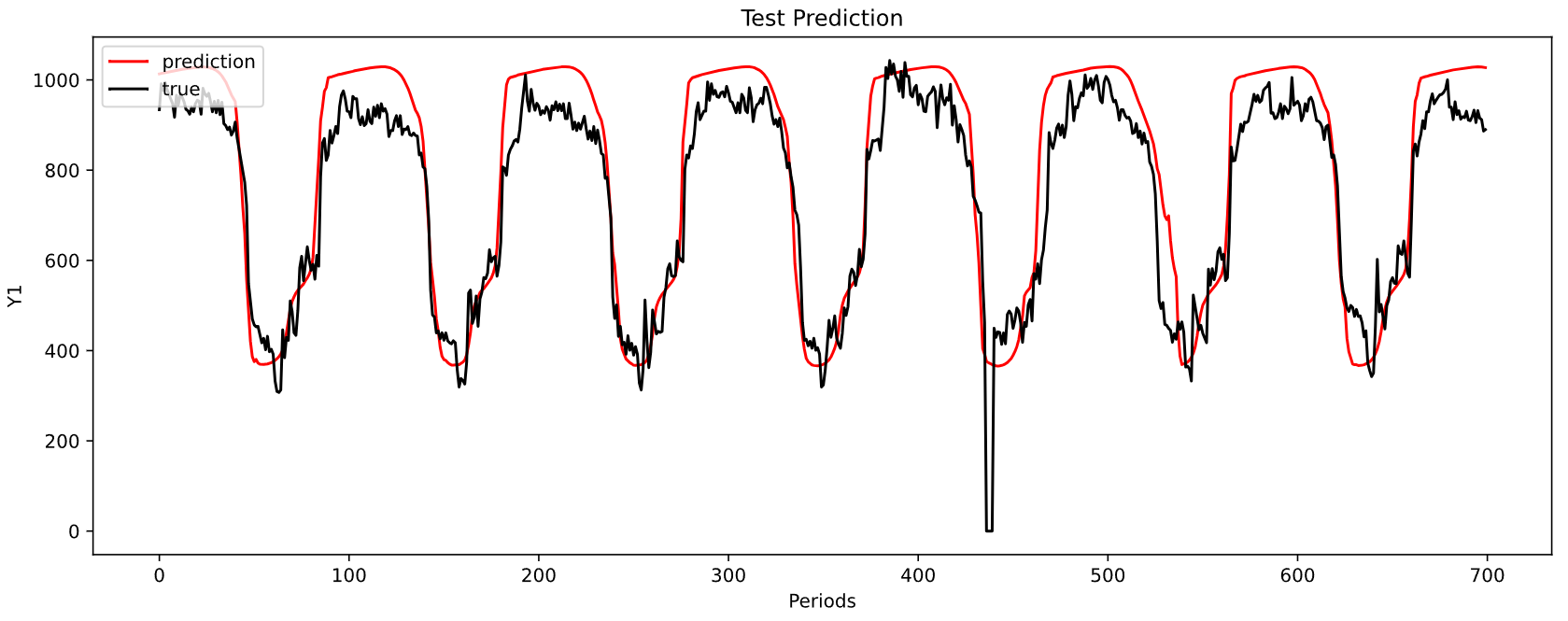
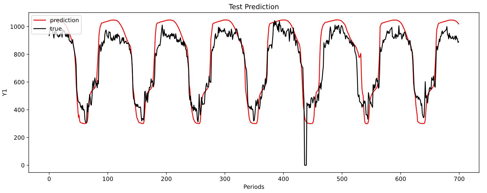
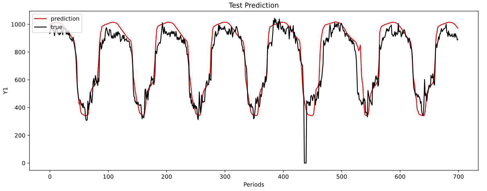
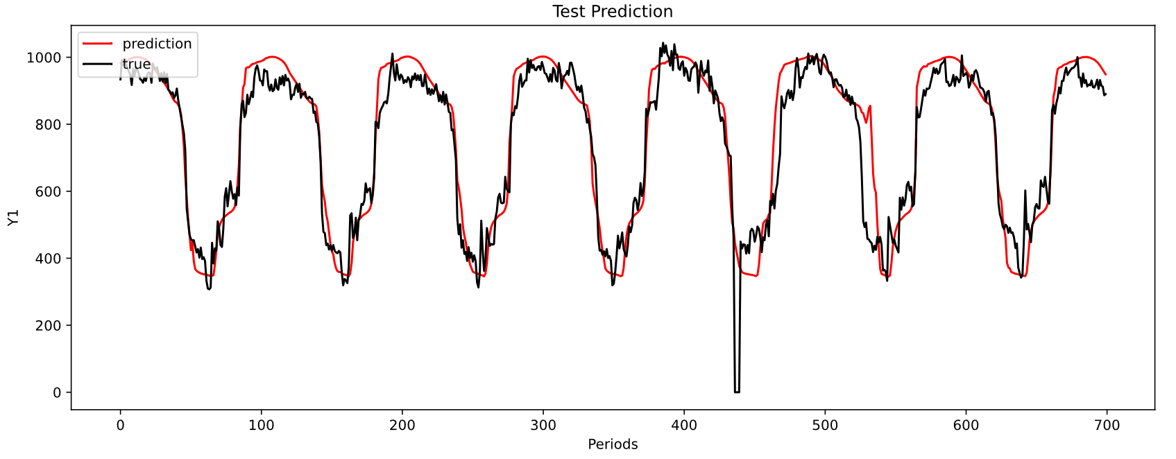
MAE: 53.98084777923004
MSE: 6170.627045824975

-----------------------------------------------------------------------------------------
| end of epoch  10 | time:  9.30s | valid loss 38.52528
-----------------------------------------------------------------------------------------
best_val_loss 38.525278732180595

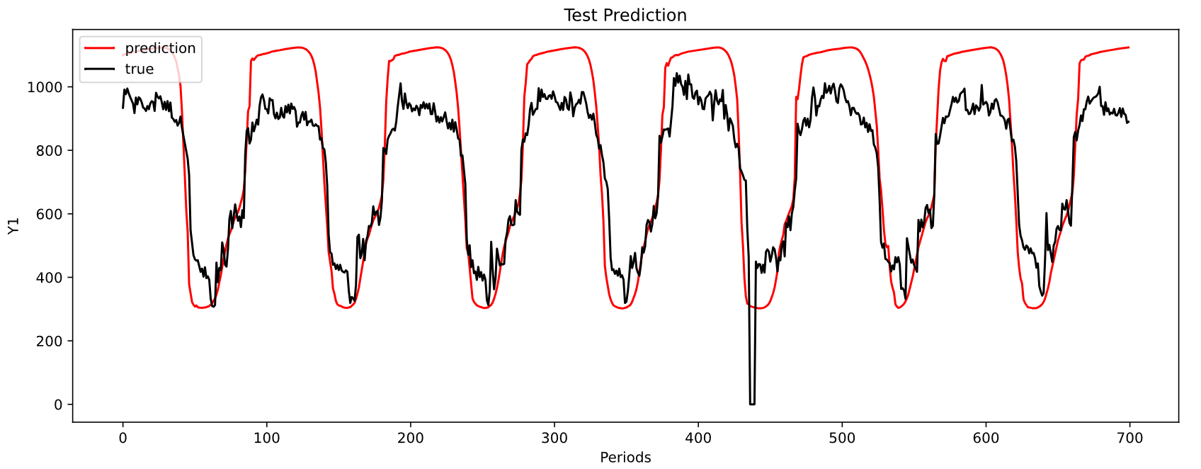
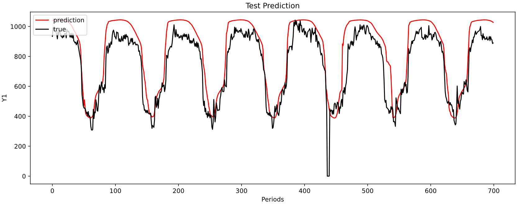
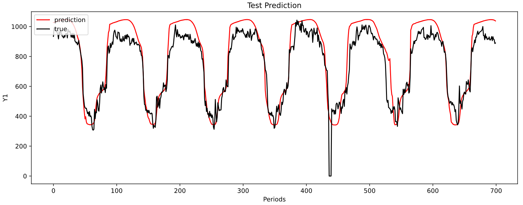
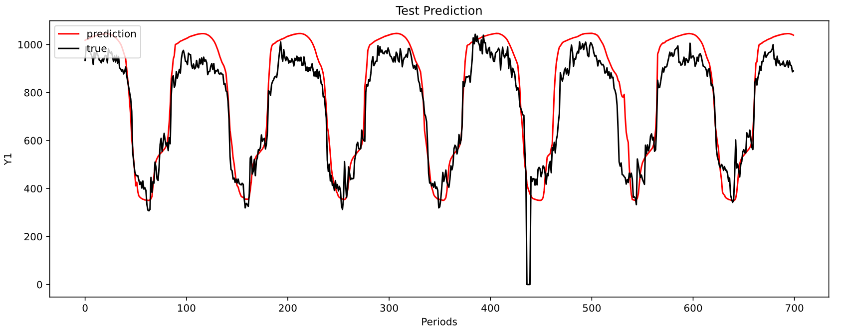
上面图形是对第一个目标序列的预测结果，最小$MAE$为$53.98$.