EE213 - Assignment 1: Fourier Analysis

In this assignment, you will:

• Use MATLAB to calculate the Fourier Series (FS) of periodic continuous signals.
• Synthesize a signal from its Fourier Series.
• Explore the Fourier Transform (FT) of continuous signals.
• Use MATLAB to compute and plot the FT.
• Explore the Discrete Time Fourier Series (DTFS) and Discrete Time
  Fourier Transform (DTFT).

The prerequisite theory for completing this assignment can be found in Lecture6: Frequency Analysis.

This description of the Assignment includes code that you can borrow and/or use to complete the tasks. You should run the sample codes in MATLAB so that you can look at the output and ensure you understand how the code works. If you understand the operation of the code samples, you will find it easier to extend this to complete the tasks in the assignment.

You should upload a single PDF file to Moodle. This PDF file should include your MATLAB code, figures, and answers to all the tasks and the questions therein.

Task 1: Fourier Series (FS) Coefficients (Analytical Method)

In Lab 1, we saw how a periodic square wave can be generated (or synthesized) by combining various complex exponential functions having different frequencies and weights. We used the Fourier series synthesis equation to achieve this.
$$x(t)=\sum _{n=-N}^N{X}_n{e}^{j2\pi n{f}_{0}t}$$
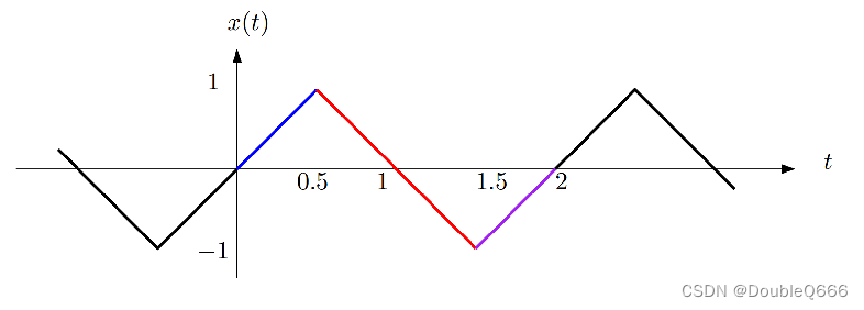
In this assignment, we will explore the Fourier series of the periodic triangular
wave shown in the following figure. The blue/red/purple portion of the signal
constitutes one full period.

Recall that the $n^{th}$ FS coefficient for a function $x(t)$ is given by
$$X_n=\frac{1}{T}{\int }_0^{T}x(t)e^{-j2\pi n{f}_{0}t}dt$$
where $T$ and $f_0=\frac{1}{T}$ are the fundamental period and frequency of $x(t)$，respectively. This is referred to as the analysis equation. Note that the weight $X_n$ represents the contribution that the complex exponential function $e^{-j2\pi n{f}_{0}t}$ with the frequency $n{f}_0$ makes to the composition of $x(t)$.

Clearly, the fundamental period and fundamental frequency of $x(t)$ are $T=2$s and $f_0=\frac{1}{2}=0.5$ Hz, respectively.

Mathematical model of $x(t)$

Before we can use the analysis equation, we need to write down a description of
one period of $x(t)$, which will be necessarily piecewise. Each coloured section is
described by a straight line over the relevant domain.

$$x(t)=\{\begin{array}{ll}2t& 0\le t\le 0.5\\ -2(t-1)& 0.5\le t\le 1.5\\ 2(t-2)& 1.5\le t\le 2\end{array}$$

Calculating FS Coefficients

Trivial Case: $\mathbf{n}=0$

• We now take the analysis equation from above and step through values of
  $n$. The simplest case is when $n=0$.
• This makes the exponent of the complex exponential $0$ (because Font metrics not found for font: .
  is $0$ when $n=0$). Thus, we have