Wireless Communications - 2.2 Transmit and Receive Signal Models & 2.3 Free-Space Path Loss

提示：文章写完后，目录可以自动生成，如何生成可参考右边的帮助文档

---

Preface

Our models are developed mainly for signals in the Ultra High Frequency (UHF) and Super High Frequency (SHF) bands, from $0.3-3\text{GHz}$ and $3-30\text{GHz}$, respectively.

All transmitted and received signals we consider are real. This is due to modulators and demodulators are built using oscillators that can generate real sinusoids only ( not complex exponentials ). Thus, the transmitted signal output from a modulator is a real signal. Similarly, the demodulator only extracts the real part of the signal at its input.

---

Transmitted Signal Model

We model the transmitted signal as
s ( t ) = ℜ { u ( t ) e j ( 2 π f c t + ϕ 0 ) } = ℜ { u ( t ) } cos ⁡ ( 2 π f c t + ϕ 0 ) − ℑ { u ( t ) } sin ⁡ ( 2 π f c t + ϕ 0 ) = x ( t ) cos ⁡ ( 2 π f c t + ϕ 0 ) − y ( t ) sin ⁡ ( 2 π f c t + ϕ 0 ) \begin{aligned} s(t) &=\Re\left\{u(t) e^{j\left(2 \pi f_{c} t+\phi_{0}\right)}\right\} \\ &=\Re\{u(t)\} \cos \left(2 \pi f_{c} t+\phi_{0}\right)-\Im\{u(t)\} \sin \left(2 \pi f_{c} t+\phi_{0}\right) \\ &=x(t) \cos \left(2 \pi f_{c} t+\phi_{0}\right)-y(t) \sin \left(2 \pi f_{c} t+\phi_{0}\right) \end{aligned} s(t)​=ℜ{u(t)ej(2πfc​t+ϕ0​)}=ℜ{u(t)}cos(2πfc​t+ϕ0​)−ℑ{u(t)}sin(2πfc​t+ϕ0​)=x(t)cos(2πfc​t+ϕ0​)−y(t)sin(2πfc​t+ϕ0​)​ where $u(t)=x(t)+jy(t)$ is a complex baseband signal with in-phase component x ( t ) = R { u ( t ) } x(t) = \mathcal{R}\{u(t)\} x(t)=R{u(t)}, quadrature component y ( t ) = ℑ { u ( t ) } y(t)=\Im\{u(t)\} y(t)=ℑ{u(t)}, bandwidth $B$, and power $P_u$. The signal $u(t)$ is called the complex envelope or complex lowpass equivalent signal of $s(t)$. This is due to the magnitude of $u(t)$ is that of $s(t)$, and the phase of $u(t)$ is that of $s(t)$ relative to the carrier frequency $f_c$ and the initial phase offset ${\varphi }_0$. This is a common representation for bandpass signals with $B<<f_c$, as it allows signal manipulation via $u(t)$ irrespective of the carrier frequency and phase. The power in the transmitted signal $s(t)$ is $P_t=P_u/2$

---

Received Signal Model

The received signal will have similar form: r ( t ) = ℜ { v ( t ) e j ( 2 π f c t + ϕ 0 ) } , r(t) = \Re \{ v(t) e^{j(2 \pi f_c t + \phi_0 )} \}, r(t)=ℜ{v(t)ej(2πfc​t+ϕ0​)}, where the complex baseband signal is $v(t)$ will depend on the channel through which $s(t)$ propagates. In particular, if $s(t)$ is transmitted through a time-invariant channel then $v(t)=u(t)\ast c(t)$, where $c(t)$ is the equivalent lowpass channel impulse response for the channel .

---

Doppler shift

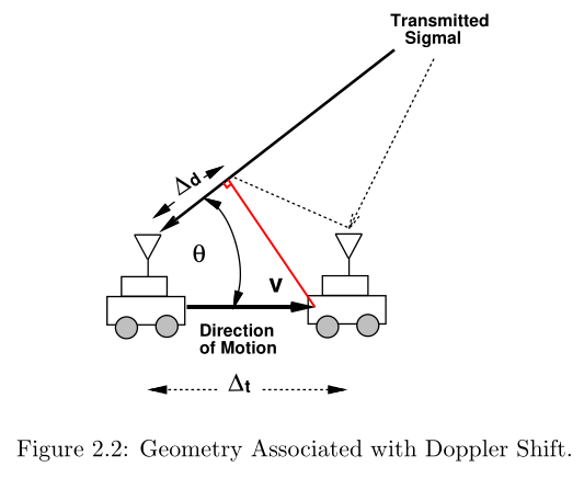
The received signal may have a Doppler shift of $$f_D=v\cos \theta /\lambda$$ associated with it, where $\theta$ is the arrival angle of the received signal relative to the direction of motion, $v$ is the receiver velocity towards the transmitter in the direction of motion, and $\lambda =c/f_c$ is the signal wavelength ($c$ is the the speed of light). The geometry associated with the Doppler shift is shown in Fig. 2.2. The Doppler shift results from the fact that transmitter or receiver movement over a short time interval $△t$ causes a slight change in distance $△d=v△t\cos \theta$ that the transmitted signal needs to travel to the receiver. The phase change due to this path length difference is $∆\phi =2\pi v∆tcos\theta /\lambda$. The Doppler frequency is then obtained from the relationship between signal frequency and phase: $$f_D=\frac{1}{2\pi }\frac{\Delta \varphi }{\Delta t}=v\cos \theta /\lambda .$$ If the receiver is moving towards the transmitter, i.e. $-\pi /2\le \theta \le \pi /2$, then the Doppler frequency is positive, otherwise it is negative.
Here, we ignore the Doppler term in the free-space and ray tracing models of this chapter, since for typical urban vehicle speeds ($60\text{mph}$) and frequency (around $1\text{GHz}$), it is less than $70\text{Hz}$.

---

Path Loss

Suppose $s(t)$ of power $P_t$ is transmitted through a given channel, with corresponding received signal $r(t)$ of power $P_r$, where $P_r$ is averaged over any random variations due to shadowing. We define the linear path loss of the channel as the ratio of transmit power to receive power: $$P_L\text{(dB)}=10{\log }_{10}\frac{P_t}{P_r}.$$

In general, path loss is a nonnegative number since the channel does not contain active elements, and thus can only attenuate the signal. The path gain in $\text{dB}$ is defined as the negative of the path loss: $$P_G=-P_L=10{\log }_{10}(P_r/P_t),$$ which is generally a negative number. With shadowing, the received power will include the effects of path loss and an additional random component due to blockage from objectives.

---

Received Signal of Free-Space Path

Consider a signal transmitted through free space to a receiver located at distance d from the transmitter. Assume there are no obstructions between the transmitter and receiver. The channel model associated with this transmission is called a Line-Of-Sight (LOS) channel, and the corresponding received signal is called the LOS signal or ray. Free-space path loss introduces a complex scale factor, resulting in the received signal:
$$r(t)=\Re \left\{\frac{\lambda \sqrt{G_l}{e}^{-j(2\pi d/\lambda )}}{4\pi d}u(t)e^{j2\pi f_{c}t}\right\},$$ where $\sqrt{G_l}$ is the product of the transmit and receive antenna Field Radiation Patterns (FRP, 场辐射图) in the LOS direction, and the phase shift $e^{-j(2\pi d/\lambda )}$ ($e^{-j(2\pi f_c\tau }$, where delay $\tau =d/c$) is due to the distance $d$ the wave travels.

---

Free-Space Path Loss

The power in the transmitted signal $s(t)$ is $P_t$, so the ratio of received to transmitted power computed by is $$\frac{P_r}{P_t}={\left[\frac{\sqrt{G_l}\lambda }{4\pi d}\right]}^2.$$ Thus, the received signal power falls off inversely proportional to the square of the distance $d$ between the transmit and receive antennas. The received signal power is also proportional to the square of the signal wavelength, so as the carrier frequency increases, the received power decreases. This dependence of received power on the signal wavelength $\lambda$ is due to the effective area of the receive antenna. However, the antenna gain of highly directional antennas can increase with frequency, so the receive power may actually increase with frequency for highly directional links.

The received power can be expressed in $\text{dBm}$ as $$P_r(\text{dBm})=P_t(\text{dBm})+10{\log }_{10}(G_l)+20lo{g}_{10}(\lambda )-20{\log }_{10}(4\pi )-20{\log }_{10}(d).$$

Free-space path loss is defined as the path loss of the free-space model: $$P_L(\text{dB})=10{\log }_{10}\frac{P_t}{P_r}=-10{\log }_{10}\frac{G_l{\lambda }^2}{(4\pi d{)}^2}.$$

The free-space path gain is thus $$P_G=-P_L=10{\log }_{10}\frac{G_l{\lambda }^2}{(4\pi d{)}^2}.$$

---