


✅作者简介:热爱科研的Matlab仿真开发者,修心和技术同步精进,matlab项目合作可私信。
🍎个人主页:Matlab科研工作室
🍊个人信条:格物致知。
更多Matlab仿真内容点击👇
⛄ 内容介绍
惯性导航系统(INS)具有完全自主性,但其导航定位精度随时间下降,因而难以长时间独立工作;全球定位系统(GPS)是全球实时高精度的导航系统,但GPS受制于人且信号易受到干扰;GPS/INS组合导航系统克服了各自缺点且组合后的导航精度高于两个系统单独工作的精度.但当GPS/INS组合系统应用到"城市峡谷"地域时,由于信号受遮挡等原因,使得GPS无法提供足够并且稳定的定位精度来修正INS的误差.此外,目前在地表以下(如城市地铁)还不能使用GPS定位技术.INS/GPS/伪卫星(PLS)组合系统是解决这些问题的一条有效途径:采用伪卫星定位技术能够增加卫星可见星的数目并改善其几何图形分布,提高导航系统的定位精度和可靠性
⛄ 部分代码
clear; close all;
addpath('filters');
addpath('helper');
addpath('thirdparty/shadedErrorBar');
% Load / process data
[T_X, omega, accel, accel_b, T_GPS, XYZ_GPS] = loadPoseGPS();
test_N = length(omega); % Sets the number of IMU readings
w = omega(1:test_N,:);
a = accel(1:test_N,:);
b_g = zeros(test_N,3);
b_a = accel_b(1:test_N,:);
t_x = T_X(1:test_N,:);
meas_used = T_GPS <= t_x(end);
t_gps = T_GPS(meas_used,:);
xyz_gps = XYZ_GPS(meas_used,:);
% -------------------------------------------------------------------------
% Initialize filter
skew = @(u) [0 -u(3) u(2);
u(3) 0 -u(1);
-u(2) u(1) 0];
ekf = EKF();
inekf = LIEKF();
% Get first observation that happens after a prediction
obsid = 1;
while(t_gps(obsid) < t_x(1))
obsid = obsid + 1;
end
pos_ekf = zeros(3,test_N);
pos_inekf = zeros(3,test_N);
std_ekf = zeros(3,test_N);
std_inekf = zeros(3,test_N);
for i = 2:test_N
if i == 1
dt = t_x;
else
dt = t_x(i) - t_x(i - 1);
%Assume gyro/IMU are basically synchronous
ekf.prediction(w(i,:)',a(i,:)',dt);
inekf.prediction(w(i,:)',a(i,:)',dt);
%Measurement update
if(i < test_N)
if(t_gps(obsid) > t_x(i) && t_x(i+1) > t_gps(obsid))
gps = [xyz_gps(obsid,1); xyz_gps(obsid,2); xyz_gps(obsid,3)];
ekf.correction(gps);
inekf.correction(gps);
obsid = min(obsid + 1, length(t_gps));
end
end
lieTocartesian(inekf)
pos_ekf(:,i) = ekf.mu(1:3);
variances = sqrt(diag(ekf.Sigma));
std_ekf(:,i) = Log(eul2rotm(ekf.mu(1:3)'));
pos_inekf(:,i) = inekf.mu(1:3,5);
vars = sqrt(diag(inekf.sigma_cart));
std_inekf(:,i) = vars(7:9);
if(mod(i,1000)==0)
fprintf('Iteration: %d/%d\n',i,test_N);
end
end
end
meas_used = T_GPS <= t_x(end);
% load gt
[~, ~, ~, ~, ~, x_gt, ~, y_gt, ~, z_gt] = loadGroundTruthAGL();
x_gt = x_gt - x_gt(1); y_gt = y_gt - y_gt(1); z_gt = z_gt - z_gt(1);
t_gt = linspace(0,T_X(end),length(x_gt));
% -------------------------------------------------------------------------
% traj plot
figure('DefaultAxesFontSize',14)
hold on;
plot3(XYZ_GPS(:,1), XYZ_GPS(:,2), XYZ_GPS(:,3),'b','LineWidth', 2);
plot3(x_gt, y_gt, z_gt,'--k','LineWidth', 4);
plot3(pos_ekf(1,:), pos_ekf(2,:), pos_ekf(3,:),'g','LineWidth', 2);
plot3(pos_inekf(1,:), pos_inekf(2,:), pos_inekf(3,:),'r','LineWidth', 2);
legend('gps', 'gt', 'EKF', 'InEKF', 'location', 'southeast')
hold off;
axis equal;
figure('DefaultAxesFontSize',14)
hold on;
plot3(XYZ_GPS(:,1), XYZ_GPS(:,2), XYZ_GPS(:,3),'b','LineWidth', 2);
plot3(x_gt, y_gt, z_gt,'--k','LineWidth', 4);
plot3(pos_inekf(1,:), pos_inekf(2,:), pos_inekf(3,:),'r','LineWidth', 2);
legend('gps', 'gt', 'InEKF', 'location', 'southeast')
hold off;
axis equal;
% -------------------------------------------------------------------------
% axis plot
figure;
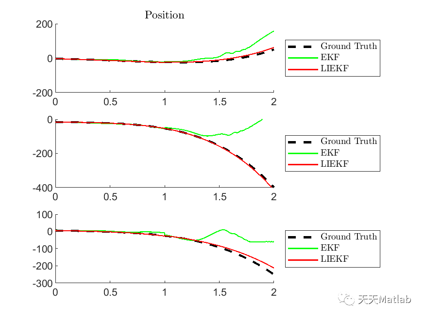
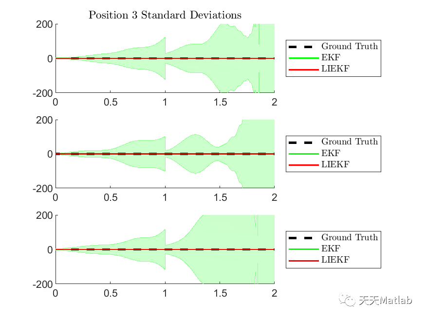
subplot(3,1,1);
hold on;
plot(t_gps, XYZ_GPS(meas_used,1), 'b', 'LineWidth', 1);
plot(t_gt, x_gt, 'k--', 'LineWidth', 2);
shadedErrorBar(T_X(1:test_N), pos_ekf(1,:), 3*std_ekf(1,:), 'lineProps', {'g', 'LineWidth', 1})
shadedErrorBar(T_X(1:test_N), pos_inekf(1,:), 3*std_inekf(1,:), 'lineProps', {'r', 'LineWidth', 1})
legend('X_{GPS}','X_{GT}','X_{EKF}', 'X_{InEKF}', 'Location', 'eastoutside');
axis([0,T_X(test_N),-200,200])
%
subplot(3,1,2);
hold on;
plot(t_gps, XYZ_GPS(meas_used,2), 'b', 'LineWidth', 1);
plot(t_gt, y_gt, 'k--', 'LineWidth', 2);
shadedErrorBar(T_X(1:test_N), pos_ekf(2,:), 3*std_ekf(2,:), 'lineProps', {'g', 'LineWidth', 1})
shadedErrorBar(T_X(1:test_N), pos_inekf(2,:), 3*std_inekf(2,:), 'lineProps', {'r', 'LineWidth', 1})
legend('Y_{GPS}','Y_{GT}','Y_{EKF}', 'Y_{InEKF}', 'Location', 'eastoutside');
axis([0,T_X(test_N),-250,350])
%
subplot(3,1,3);
hold on;
plot(t_gps, XYZ_GPS(meas_used,3), 'b', 'LineWidth', 1);
plot(t_gt, z_gt, 'k--', 'LineWidth', 2);
shadedErrorBar(T_X(1:test_N), pos_ekf(3,:), 3*std_ekf(3,:), 'lineProps', {'g', 'LineWidth', 1})
shadedErrorBar(T_X(1:test_N), pos_inekf(3,:), 3*std_inekf(3,:), 'lineProps', {'r', 'LineWidth', 1})
legend('Z_{GPS}','Z_{GT}','Z_{EKF}', 'Z_{InEKF}', 'Location', 'eastoutside');
axis([0,T_X(test_N),-30,60])
function u = unskew(ux)
u(1,1) = -ux(2,3);
u(2,1) = ux(1,3);
u(3,1) = -ux(1,2);
end
function w = Log(R)
w = unskew(logm(R));
end
⛄ 运行结果


⛄ 参考文献
[1]罗汶锋. 基于自适应簇的卡尔曼滤波定位跟踪算法[D]. 华南理工大学.
❤️ 关注我领取海量matlab电子书和数学建模资料
❤️部分理论引用网络文献,若有侵权联系博主删除


 7039
7039


 被折叠的 条评论
为什么被折叠?
被折叠的 条评论
为什么被折叠?
 到【灌水乐园】发言


