基于Matlab实现交通系统监控应用的雷达传感器信号采集和多维 FFT 处理

✅作者简介：热爱科研的Matlab仿真开发者，修心和技术同步精进，matlab项目合作可私信。

🍎个人主页：Matlab科研工作室

🍊个人信条：格物致知。

更多Matlab仿真内容点击👇

智能优化算法       神经网络预测       雷达通信       无线传感器        电力系统

信号处理              图像处理               路径规划       元胞自动机        无人机 

⛄ 内容介绍

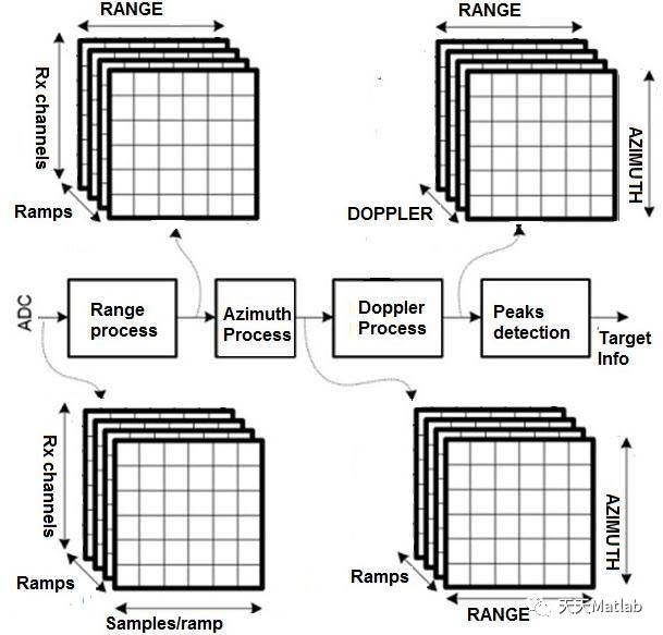
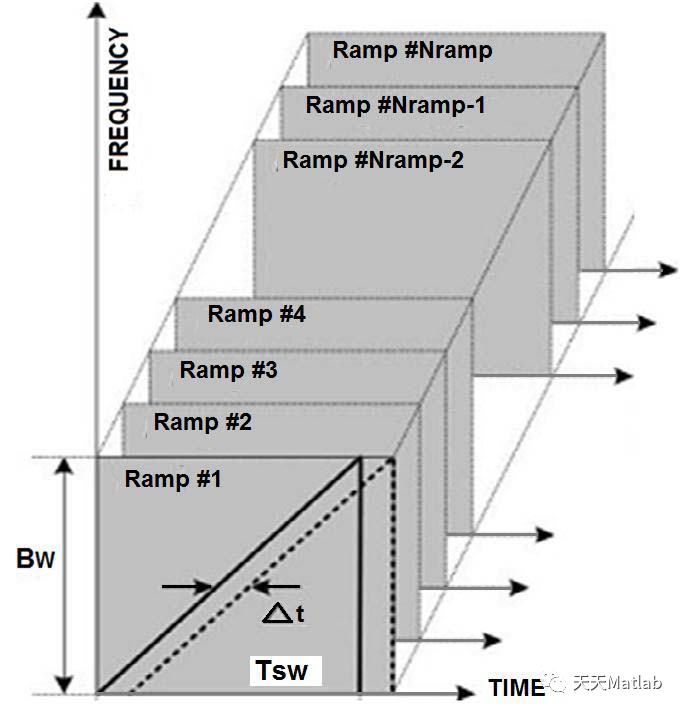
本文介绍了一种无线电探测与测距（雷达）传感器信号采集与处理平台的设计与测试。雷达传感器实时运行，适用于运输系统中的监控应用。它包括一个带有在 X 波段工作的连续波调频收发器的前端，带有一个发射器和多个接收器，以及一个多通道高速 A/D 转换器。传感器信号处理和与外部主机的数据通信任务由现场可编程门阵列管理。信号处理链包括感兴趣区域选择、多维快速傅里叶变换、峰值检测、警报决策逻辑、数据校准和诊断。通过将雷达传感平台配置为低功耗模式（7 dBm 发射功率），可以检测覆盖范围高达 300 米和 30 厘米分辨率的静止和移动目标。通过添加一个额外的 34.5 dBm 功率放大器，测量范围可以增加到 2 公里。雷达传感平台可配置为最大检测速度为 200 公里/小时，分辨率为 1.56 公里/小时，或者最高可达 50 公里/小时，分辨率为 0.4 公里/小时。跨量程分辨率取决于接收通道数；可以在雷达传感器的交叉范围分辨率与其复杂性和功耗之间找到权衡。关于监视雷达传感器和光检测与测距的最新技术水平，所提出的解决方案代表了其高可配置性以及可以在覆盖距离和功耗方面找到的更好权衡。​

⛄ 部分代码

%% Ali Karimzadeh Esfahani

% please run this file, it will call FMCW_radar function

clc

close all

clear all

[y_lk1, ~, ~, ~, ~, ~, cross_range_res1] = FMCW_radar(100, -50/3.6, -60*pi/180); 

[y_lk2, Dres, Dmax, Vres, Vmax, theta_res, cross_range_res2] = FMCW_radar(200, 75/3.6, 45*pi/180);

y_lk = y_lk1 + y_lk2;

%% FFT and FFTSHIFT

Y = abs(fftshift(fftn(y_lk,2.^nextpow2(size(y_lk)))));

YY = log(Y(floor((length(Y)/2)+1):end,:,:)+1);

max1 = max(YY,[],'all');

max2 = max(YY(YY<max(YY,[],'all')),[],'all');

[x1, y1, a1] = ind2sub(size(YY), find(YY==max1));

[x2, y2, a2] = ind2sub(size(YY), find(YY==max2));

Y = abs(fftshift(fftn(y_lk,(2.^nextpow2(size(y_lk))).*[1,1,8])));

YY = Y(floor((length(Y)/2)+1):end,:,:);

logYY = log(YY+1);

a1 = a1 * 8;

a2 = a2 * 8;

%% FFT 2D part

% heatmap(mat2gray(Y(:,:,1)),'Colormap', jet); grid off

figure('Name','2D ffts','WindowState','maximized')

subplot(2,2,1);

% for plot of range-Doppler spectrum (2-D FFT magnitude)

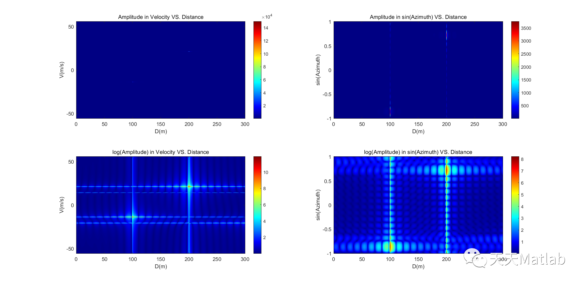
imagesc([0,Dmax],[-Vmax,Vmax],YY(:,:,floor(size(Y,3)/2)).'); 

set(gca,'YDir','normal') % flips the y-axis! (to see increasing values, not decreasing)

colorbar % display colorbar

colormap jet

title('Amplitude in Velocity VS. Distance')

xlabel('D(m)')

ylabel('V(m/s)')

subplot(2,2,2);

% for plot of range-Doppler spectrum (2-D FFT magnitude)

imagesc([0,Dmax],[-1,1],squeeze(YY(:,floor(size(Y,2)/2),:)).'); 

set(gca,'YDir','normal') % flips the y-axis! (to see increasing values, not decreasing)

colorbar % display colorbar

colormap jet

title('Amplitude in sin(Azimuth) VS. Distance')

xlabel('D(m)')

ylabel('sin(Azimuth)')

subplot(2,2,3);

% for log plot of range-Doppler spectrum (2-D FFT magnitude)

imagesc([0,Dmax],[-Vmax,Vmax],logYY(:,:,floor(size(Y,3)/2)).'); 

set(gca,'YDir','normal') % flips the y-axis! (to see increasing values, not decreasing)

colorbar % display colorbar

colormap jet

title('log(Amplitude) in Velocity VS. Distance')

xlabel('D(m)')

ylabel('V(m/s)')

subplot(2,2,4);

% for log plot of range-Doppler spectrum (2-D FFT magnitude)

imagesc([0,Dmax],[-1,1],squeeze(logYY(:,floor(size(Y,2)/2),:)).'); 

set(gca,'YDir','normal') % flips the y-axis! (to see increasing values, not decreasing)

colorbar % display colorbar

colormap jet

title('log(Amplitude) in sin(Azimuth) VS. Distance')

xlabel('D(m)')

ylabel('sin(Azimuth)')

% for plotting on the same plot two rows or two columns from a

% range-Doppler spectrum

%% FFT 1D part and finding the maximum

figure('Name','1D ffts','WindowState','maximized')

title('1D fft')

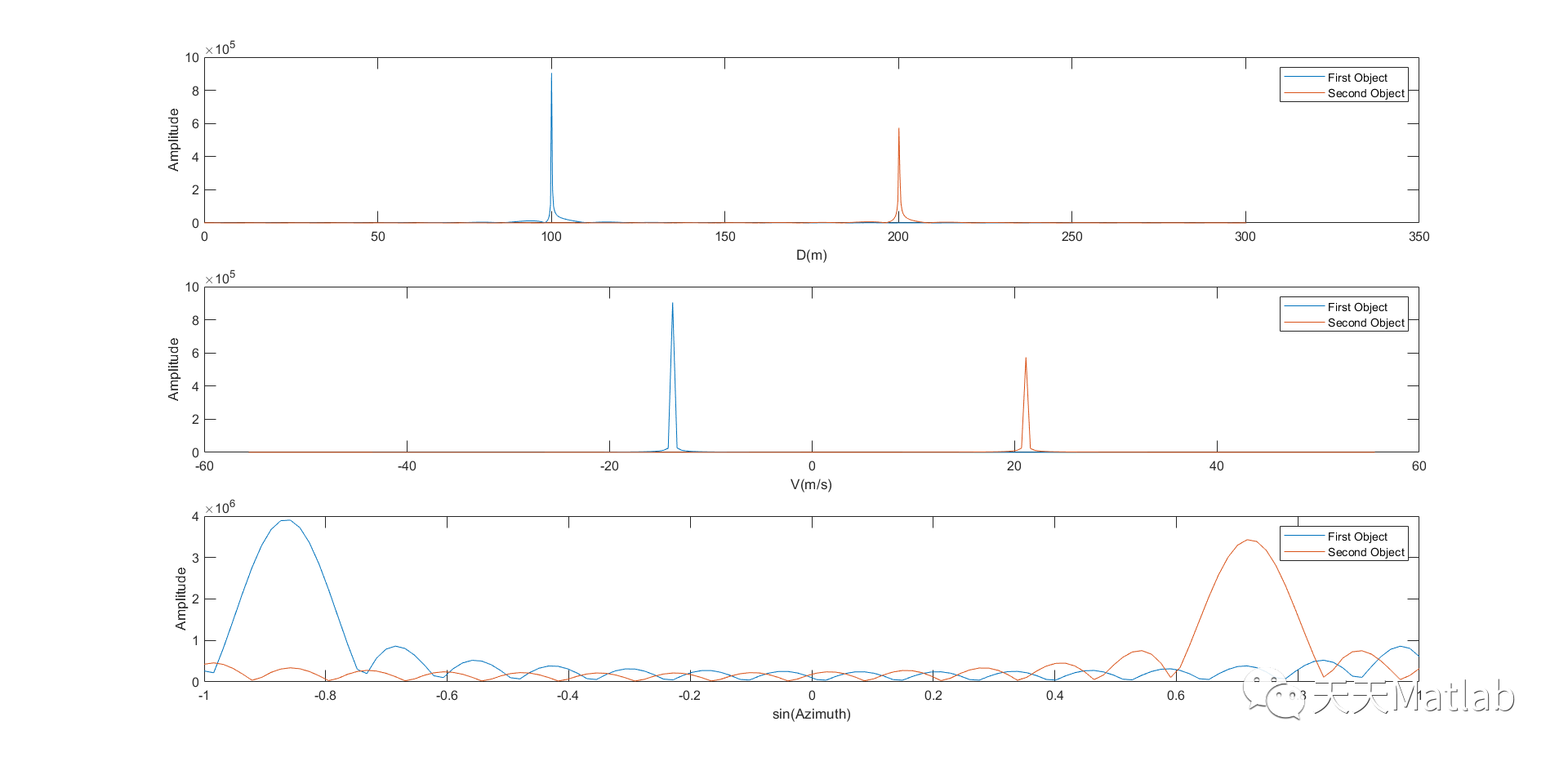
subplot(3,1,1);

plt_d = linspace(0,Dmax,length(Y)/2);

plot(plt_d, YY(:,y1,a1))

D1 = plt_d(squeeze(YY(:,y1,a1))==max(squeeze(YY(:,y1,a1))));

hold on;

D2 = plt_d(squeeze(YY(:,y2,a2))==max(squeeze(YY(:,y2,a2))));

plot(plt_d, YY(:,y2,a2))

xlabel('D(m)')

ylabel('Amplitude')

legend('First Object', 'Second Object')

subplot(3,1,2);

plt_v = linspace(-Vmax,Vmax,size(Y,2));

V1 = plt_v(squeeze(YY(x1,:,a1))==max(squeeze(YY(x1,:,a1))));

plot(plt_v, YY(x1,:,a1))

hold on;

V2 = plt_v(squeeze(YY(x2,:,a2))==max(squeeze(YY(x2,:,a2))));

plot(linspace(-Vmax,Vmax,size(Y,2)), YY(x2,:,a2))

xlabel('V(m/s)')

ylabel('Amplitude')

legend('First Object', 'Second Object')

subplot(3,1,3);

plt_a = linspace(-1,1,size(Y,3));

A1 = plt_a(squeeze(YY(x1,y1,:))==max(squeeze(YY(x1,y1,:))));

plot(plt_a, squeeze(YY(x1,y1,:)))

hold on;

A2 = plt_a(squeeze(YY(x2,y2,:))==max(squeeze(YY(x2,y2,:))));

plot(plt_a, squeeze(YY(x2,y2,:)))

xlabel('sin(Azimuth)')

ylabel('Amplitude')

legend('First Object', 'Second Object')

%% FFT Polar and Objects locations

figure('Name','polar fft','WindowState','maximized')

axis equal

image = squeeze(log(Y(floor((length(Y)/2)+1):end,round(mean([y1,y2])),:)+1));

xy_image = zeros(floor(Dmax/Dres), floor(Dmax/Dres/2));

for i = 1 : size(xy_image, 1)

    for j = 1 : size(xy_image, 2)

        xi=i*Dres*2-Dmax;

        yi=j*Dres*2;

        di=sqrt(xi^2+yi^2);

        if di<Dmax

            xy_image(i,j) = image(round(di*size(image, 1)/Dmax),ceil((xi/di+1)*size(image, 2)/2));

        end

    end

end

imagesc([-Dmax,Dmax],[0,Dmax],xy_image.'); 

set(gca,'YDir','normal') % flips the y-axis! (to see increasing values, not decreasing)

colorbar % display colorbar

colormap jet

hold on; % Prevent image from being blown away.

plot(D1*A1, D1*cos(asin(A1)),'ro', 'MarkerSize', 10, 'MarkerFaceColor', 'r');

hold on; % Prevent image from being blown away.

plot(D2*A2, D2*cos(asin(A2)),'mo', 'MarkerSize', 10, 'MarkerFaceColor', 'm');

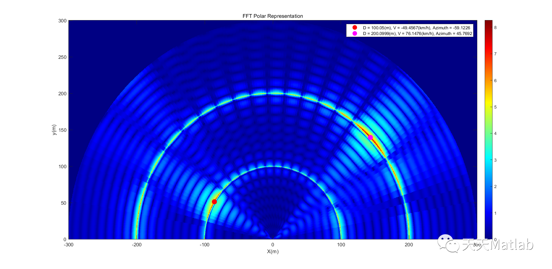
legend('D = '+string(D1)+'(m), V = '+string((V1)*3.6)+'(km/h), Azimuth = '+string(asind(A1)), ...

    'D = '+string(D2)+'(m), V = '+string((V2)*3.6)+'(km/h), Azimuth = '+string(asind(A2)));

title('FFT Polar Representation')

xlabel('X(m)')

ylabel('y(m)')

⛄ 运行结果

⛄ 参考文献

⛳️ 代码获取关注我

❤️部分理论引用网络文献，若有侵权联系博主删除

❤️ 关注我领取海量matlab电子书和数学建模资料