基于Matlab模拟时变瑞利衰落信道中的差分放大转发中继

✅作者简介：热爱科研的Matlab仿真开发者，修心和技术同步精进，matlab项目合作可私信。

🍎个人主页：Matlab科研工作室

🍊个人信条：格物致知。

更多Matlab仿真内容点击👇

智能优化算法       神经网络预测       雷达通信       无线传感器        电力系统

信号处理              图像处理               路径规划       元胞自动机        无人机 

⛄ 内容介绍

1 算法原理

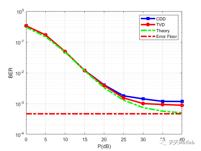
This paper considers the performance of differential amplify-and-forward (D-AF) relaying over time-varying Rayleigh fading channels. Using the auto-regressive time-series model to characterize the time-varying nature of the wireless channels, new weights for the maximum ratio combining (MRC) of the received signals at the destination are proposed. Expression for the pair-wise error probability (PEP) is provided and used to obtain an approximation of the total average bit error probability (BEP). The obtained BEP approximation clearly shows how the system performance depends on the auto-correlation of the direct and the cascaded channels and an irreducible error floor exists at high signal-to-noise ratio (SNR). Simulation results also demonstrate that, for fast-fading channels, the new MRC weights lead to a better performance when compared to the classical combining scheme. Our analysis is verified with simulation results in different fading scenarios.

2 算法流程

Differential Amplify-and-Forward (DAF) relaying is a technique used in wireless communication systems to improve performance in time-varying Rayleigh fading channels. In DAF relaying, the relay node receives the modulated signal from the source node differentially and amplifies it before forwarding it to the destination node.

Here is a general overview of the DAF relaying process in time-varying Rayleigh fading channels:

1. Source-to-relay transmission:

   • The source node transmits a modulated signal in the first time slot.

   • The signal experiences fading and attenuation as it propagates through the channel.

2. Relay amplification:

   • The relay node receives the signal differentially, comparing it with a local delayed version of the received signal from the previous time slot.

   • The relay node amplifies the differentially-encoded signal to enhance its strength.

3. Relay-to-destination transmission:

   • The relay node forwards the amplified signal to the destination node in the next time slot.

   • The signal undergoes further fading and attenuation during transmission.

4. Destination reception:

   • The destination node receives the relayed signal and demodulates it to recover the transmitted data.

Key advantages of DAF relaying in time-varying Rayleigh fading channels include:

1. Diversity gain: The differential encoding at the relay provides diversity gain, allowing for better performance in fading channels.

2. Simplified processing: DAF relaying reduces the need for coherent phase and timing synchronization between the source and relay nodes.

3. Robustness to fading variations: Differential processing mitigates the impact of channel fading variations over consecutive time slots.

It's worth noting that the specific implementation and performance of DAF relaying may vary depending on the system design, modulation scheme, fading characteristics, and other factors. Channel estimation, power control, and cooperation strategies can also be incorporated to further enhance the performance of DAF relaying in time-varying Rayleigh fading channels.

⛄ 部分代码

%% Simulation of the following paper

% M. R. Avendi and Ha H. Nguyen, "Differential Amplify-and-Forward relaying

% in time-varying Rayleigh fading channels," IEEE Wireless Communications 

% and Networking Conference (WCNC), Shanghai, China, 2013,

clc

close all

clear all

addpath('functions')

%%

% MPSK modulation

M=2;

Ns=1E5;% number of symbols

Ptot_dB=0:5:40;% SNR scan

Ptot=10.^(Ptot_dB/10);

N0=1; % noise power

% number of Relays

R=1;

% channel distance between channel uses

ch_dis=0; % for symbol-by-symbol n=R

%  scenarios

vfsd=[.001,.01,.05];

vfsr=[.001,.01,.05];

vfrd=[.001,.001,0.01];

% select the scenario

scenario=3;

% normalized Dopplers

fsd=vfsd(scenario);

fsr=vfsr(scenario);

frd=vfrd(scenario);

% auto-correlations

[alfa_sd,alfa]=auto_corr(fsd,fsr,frd,ch_dis);

% power allocation

%[P0,P1]=opt_pow(Ptot,fsd,fsr,frd,M,n);

P0=Ptot./2;

Pi=Ptot./2./R;

Ai2= Pi./(P0+N0);

% CDD power allocation

if M==2, c=.5; else c=.5; end

P0_cdd=c*Ptot;

Pi_cdd=(1-c)*Ptot./R;

Ai2_cdd= Pi_cdd./(P0_cdd+N0);

% this loop scans the SNR range

for ind=1:length(Ptot)

nbits=0;%total number of info sent

err_cdd=0;% error counter 

err_tvd=0;% error counter

clc

Ptot_dB(ind)

% this loop keeps going to get a certain amount of errors

ERR_TH=100;

while err_cdd<ERR_TH || err_tvd<ERR_TH

% info bits

xb=bits(log2(M)*Ns);

%binary  to MPSK

v=bin2mpsk(xb,M);

% DPSK modulation

s=diff_encoder(v);

Nd=length(s);

% S-D channel

hsd=flat_cos(Nd,fsd,ch_dis);

% S-R and R-D channels

for k=1:R

hsr(k,:)=flat_cos(Nd,fsr,ch_dis);

hrd(k,:)=flat_cos(Nd,frd,ch_dis);

end

% AWGN noise CN(0,N0)

z_sd=cxn(Nd,N0);

for k=1:R

z_sr(k,:)=cxn(Nd,N0);

z_rd(k,:)=cxn(Nd,N0);

end

%--------------------------------------- received signals

% CDD power allocation

y_sd_cdd=sqrt(P0_cdd(ind))*hsd.*s+z_sd;

for k=1:R

y_sr_cdd(k,:)=sqrt(P0_cdd(ind))*hsr(k,:).*s+z_sr(k,:);

y_rd_cdd(k,:)=sqrt(Ai2_cdd(ind))*hrd(k,:).*y_sr_cdd(k,:)+z_rd(k,:);

end

% propossed power allocation for time-varying

y_sd=sqrt(P0(ind))*hsd.*s+z_sd;

for k=1:R

y_sr_tvd(k,:)=sqrt(P0(ind))*hsr(k,:).*s+z_sr(k,:);

y_rd_tvd(k,:)=sqrt(Ai2(ind))*hrd(k,:).*y_sr_tvd(k,:)+z_rd(k,:);

end

% ---------------------------------------- MRC combining

% classical weights

a0_cdd=1/2;

ai_cdd=1/(1+Ai2_cdd(ind))/2;

vh_cdd=a0_cdd*diff_detector(y_sd_cdd);

for k=1:R

vh_cdd=vh_cdd+ai_cdd*diff_detector(y_rd_cdd(k,:));

end

% propossed weights for time-varying

[at1,at2]=mrc_gains(P0(ind),Ai2(ind),alfa_sd,alfa);

vh_tvd=at1*diff_detector(y_sd);

for k=1:R

vh_tvd=vh_tvd+at2*diff_detector(y_rd_tvd(k,:));

end

% selection combining

%vh2=max((diff_detector(y_sd)),(diff_detector(y_rd)));

% binary detection

bh_cdd=mpsk2bin(vh_cdd,M);

bh_tvd=mpsk2bin(vh_tvd,M);

% error count

err_cdd=err_cdd+sum(abs(xb-bh_cdd));

err_tvd=err_tvd+sum(abs(xb-bh_tvd));

nbits=log2(M)*Ns+nbits;

end

% compute practical BER 

BER_cdd(ind)=err_cdd/nbits;% coperative

BER_tvd(ind)=err_tvd/nbits;% coperative

end

% SER

Pu=Pupper(P0,Ai2,fsd,fsr,frd,M,ch_dis);

Ps=Ps_num_int(P0,Ai2,fsd,fsr,frd,M,ch_dis);

Psf=Ps_floor(fsd,fsr,frd,M,ch_dis);

% upper bound

Pb_ub=Pu./log2(M);

% theoretical bit error rate

Pb_theory=Ps./log2(M);

% error floor

Pbf=Psf/log2(M)*ones(1,length(P0));

%% plot 

lcm=['b-s';'r-o';'k:>';'g-.';'y-*'];

figure

semilogy(Ptot_dB,BER_cdd,lcm(1,:),'LineWidth',3,'MarkerSize',5);

hold on

semilogy(Ptot_dB,BER_tvd,lcm(2,:),'LineWidth',3,'MarkerSize',5);

%semilogy(Ptot_dB,Pb_ub,lcm(3,:),'LineWidth',3,'MarkerSize',5);

semilogy(Ptot_dB,Pb_theory,lcm(4,:),'LineWidth',3,'MarkerSize',5);

semilogy(Ptot_dB,Pbf,'r-.','LineWidth',3,'MarkerSize',5);

legend('CDD','TVD','Theory','Error Floor')

grid on

xlabel('P(dB)')

ylabel('BER')

⛄ 运行结果

⛄ 参考文献

M. R. Avendi and Ha H. Nguyen, "Differential Amplify-and-Forward relaying in time-varying Rayleigh fading channels," IEEE Wireless Communications and Networking Conference (WCNC), Shanghai, China, 2013,

🍅 仿真咨询

1.卷积神经网络（CNN）、LSTM、支持向量机（SVM）、最小二乘支持向量机（LSSVM）、极限学习机（ELM）、核极限学习机（KELM）、BP、RBF、宽度学习、DBN、RF、RBF、DELM实现风电预测、光伏预测、电池寿命预测、辐射源识别、交通流预测、负荷预测、股价预测、PM2.5浓度预测、电池健康状态预测、水体光学参数反演、NLOS信号识别、地铁停车精准预测、变压器故障诊断

2.图像识别、图像分割、图像检测、图像隐藏、图像配准、图像拼接、图像融合、图像增强、图像压缩感知

3.旅行商问题（TSP）、车辆路径问题（VRP、MVRP、CVRP、VRPTW等）、无人机三维路径规划、无人机协同、无人机编队、机器人路径规划、栅格地图路径规划、多式联运运输问题、车辆协同无人机路径规划

4.无人机路径规划、无人机控制、无人机编队、无人机协同、无人机任务分配

5.传感器部署优化、通信协议优化、路由优化、目标定位

6.信号识别、信号加密、信号去噪、信号增强、雷达信号处理、信号水印嵌入提取、肌电信号、脑电信号

7.生产调度、经济调度、装配线调度、充电优化、车间调度、发车优化、水库调度、三维装箱、物流选址、货位优化

8.微电网优化、无功优化、配电网重构、储能配置

9.元胞自动机交通流 人群疏散 病毒扩散 晶体生长

⛳️ 代码获取关注我

❤️部分理论引用网络文献，若有侵权联系博主删除

❤️ 关注我领取海量matlab电子书和数学建模资料