如何处理异常值和强影响点？(python)

异常值分为两种情况：因变量y异常和自变量x异常。

1 因变量y异常

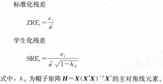
标准化残差使残差具有可比性，可通过3σ原则判定异常值，但没有解决方差不等问题。

学生化残差解决了方差不等问题，但当观测值中存在异常值时，普通残差、标准化残差、学生化残差不再适用。

因为异常值会把回归线拉向自身，使异常值本身的残差减少，而其余观测值的残差增大，这时3σ原则不能准确分辨出异常值，解决方法是改用删除残差。

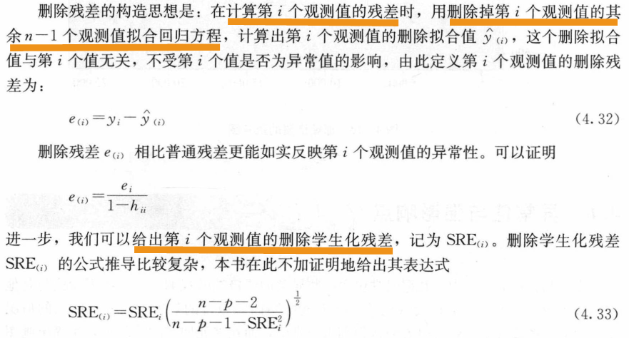
|SRE(i)| 大于3的观测值即判定为异常值。

python 实现：

# https://stackoverflow.com/questions/59466607/calculate-studentized-deletion-residuals-and-outlier-test-for-the-predictions
def internally_studentized_residual(X,Y,y_hat):
    """
    Calculate studentized residuals internal
    Parameters
    ______________________________________________________________________
    X:            List
                  Variable x-axis
    Y:            List
                  Response variable of the X 
    y_hat:        List
                  Predictions of the response variable with the given X
    Returns
    ______________________________________________________________________
    Dataframe :   List
                  Studentized Residuals   
    """
#     print(len(Y))
    X = np.array(X, dtype=float)
    Y = np.array(Y, dtype=float)
    y_hat = np.array(y_hat,dtype=float)
    mean_X = np.mean(X)
    mean_Y = np.mean(Y)
    n = len(X)
#     print(X.shape,Y.shape,y_hat.shape)
    residuals = Y - y_hat
    X_inverse = np.linalg.pinv(X.reshape(-1,1))[0]
    h_ii = X_inverse.T * X
    Var_e = math.sqrt(sum((Y - y_hat) ** 2)/(n-2))
    SE_regression = Var_e/((1-h_ii) ** 0.5)
    studentized_residuals = residuals/SE_regression
    return studentized_residuals

def deleted_studentized_residual(X,Y,y_hat):
    """
    Calculate studentized residuals external
    Parameters
    ______________________________________________________________________
    X:            List
                  Variable x-axis
    Y:            List
                  Response variable of the X 
    y_hat:        List
                  Predictions of the response variable with the given X
    Returns
    ______________________________________________________________________
    Dataframe :   List
                  Studentized Residuals External  
    """
    #formula from https://newonlinecourses.science.psu.edu/stat501/node/401/
    r = internally_studentized_residual(X,Y,y_hat)
    n = len(r)
    return [r_i*math.sqrt((n-2-1)/(n-2-r_i**2)) for r_i in r]

def outlier_test(X,Y,y_hat,alpha=0.1):
    """
    outlier test for the points
    Parameters
    ______________________________________________________________________
    X:            List
                  Variable x-axis
    Y:            List
                  Response variable of the X 
    y_hat:        List
                  Predictions of the response variable with the given X
    alpha:        float
                  alpha value for multiple test
    Returns
    ______________________________________________________________________
    Dataframe :   studentized, unadjusted p values and benferroni multiple 
                  test dataframe  
    """
    resid = deleted_studentized_residual(X,Y,y_hat)
    df = len(X) - 1 
    p_vals = stats.t.sf(np.abs(resid),df) * 2
    bonf_test = multipletests(p_vals,alpha,method="bonf")
    df_result = pd.DataFrame()
    df_result.loc[:,"student_resid"] = resid
    df_result.loc[:,"unadj_p"] = p_vals
    df_result.loc[:,"bonf(p)"] = bonf_test[1]
    df_result.index = X.index
    return df_result

2 因变量x异常

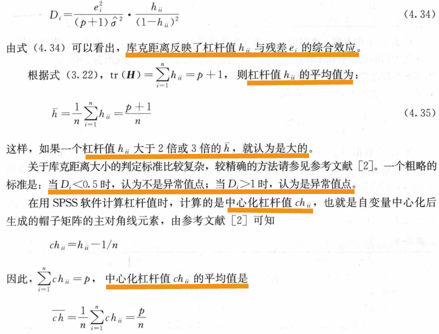
上面式子中的hii为帽子矩阵中主对角的第i个元素，是调节ei方差大小的杠杆，因此hii被称为第i个观测值的杠杆值。

较大的杠杆值残差偏小，因为杠杆值大的观测点远离样本中心，能够把回归方程拉向自身，因而把杠杆值大的样本点称为强影响点。

强影响点并不一定是y的异常值点，因此强影响点并不总会对回归方程造成不良影响，但对回顾效果有较强的影响，需重视：

• 在实际问题中，因变量与自变量的线性关系只是在一定范围内成立，强影响点远离样本中心，因变量与自变量之间可能不再是线性函数关系，因而在选择回归函数形式时，要侧重于强影响点
• 即使线性回归形式成立，但是强影响点远离样本中心，能够把回归方程拉向自身，使回归方程产生偏移

由于强影响点并不一定是y的异常值点，因此不能单纯根据杠杆值hii的大小判断强影响点是否异常。为此，引入库克距离，用来判断强影响点是否为y的异常值点。其计算公式为：

python 实现：

# https://www.statology.org/cooks-distance-python/
import pandas as pd
import statsmodels.api as sm
import numpy as np
np.set_printoptions(suppress=True)
import matplotlib.pyplot as plt

"""Step 1: Enter the Data"""
#create dataset
df = pd.DataFrame({'x': [8, 12, 12, 13, 14, 16, 17, 22, 24, 26, 29, 30],
                   'y': [41, 42, 39, 37, 35, 39, 45, 46, 39, 49, 55, 57]})

"""Step 2: Fit the Regression Model"""
#define response variable
y = df['y']

#define explanatory variable
x = df['x']

#add constant to predictor variables
x = sm.add_constant(x)

#fit linear regression model
model = sm.OLS(y, x).fit() 

"""Step 3: Calculate Cook’s Distance"""
#create instance of influence
influence = model.get_influence()

#obtain Cook's distance for each observation
cooks = influence.cooks_distance

#display Cook's distances
print(cooks)

# displays an array of values for Cook’s distance for each observation followed by an array of corresponding p-values
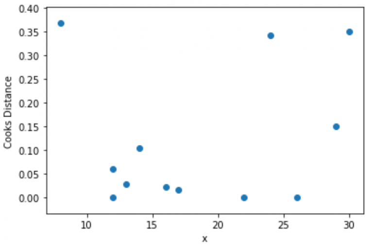
(array([0.368, 0.061, 0.001, 0.028, 0.105, 0.022, 0.017, 0.   , 0.343,
        0.   , 0.15 , 0.349]),
 array([0.701, 0.941, 0.999, 0.973, 0.901, 0.979, 0.983, 1.   , 0.718,
        1.   , 0.863, 0.713]))

"""Step 4: Visualize Cook’s Distances"""
plt.scatter(df.x, cooks[0])
plt.xlabel('x')
plt.ylabel('Cooks Distance')
plt.show()