


摘要: 分享对论文的理解, 原文见 Peng Jin, Xitong Zhang, Yinpeng Chen, Sharon Xiaolei Huang, Zicheng Liu, Youzuo Lin, Unsupervised learning of full-waveform inversion: connecting CNN and partial differential equation in a loop.
论文发表于计算机方面的顶会 ICLR.
1. 论文贡献
- 提出一种无监督的 FWI 网络. 其实说 “无监督” 有些牵强, 因为它的监督信息 (速度模型) 通过正演获得的数据, 与原始数据之间可以计算损失.
- 做了一个数据集 OpenFWI, 在另一篇论文里面专门介绍. 对于这个方向的研究人员非常重要.
2. 论文工作
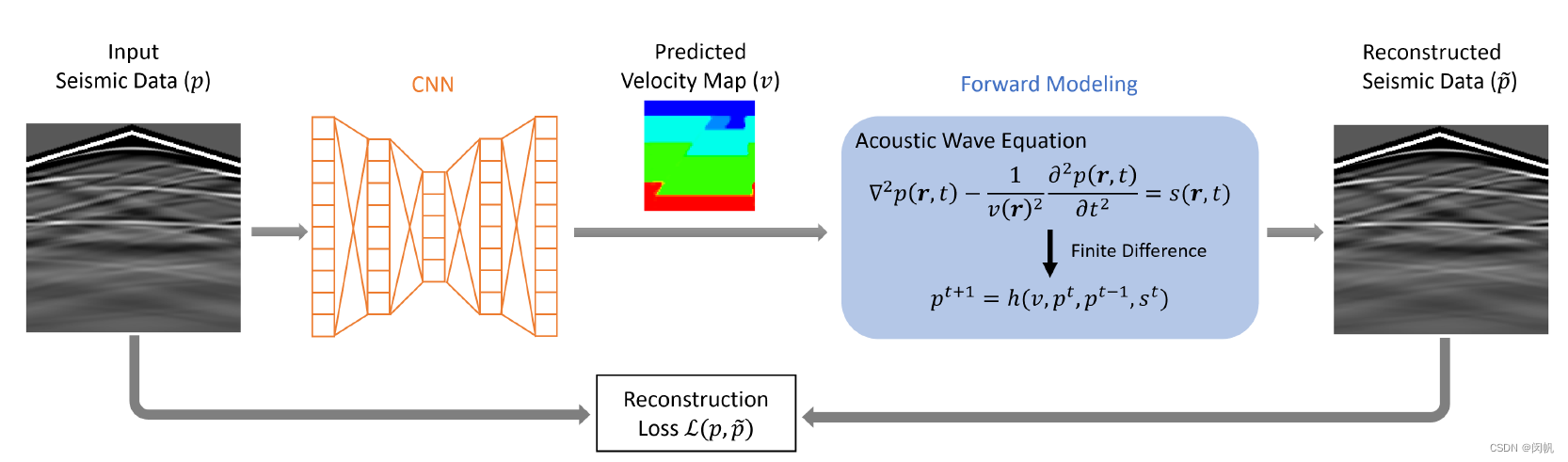
- 反演用 CNN
- 正演用 PDE
2.1 正演模型
∇
2
p
(
r
,
t
)
−
1
v
(
r
)
2
∂
2
p
(
r
,
t
)
∂
t
2
=
s
(
r
,
t
)
(1)
\nabla^2 p(\mathbf{r}, t) - \frac{1}{v(\mathbf{r})^2} \frac{\partial^2 p(\mathbf{r}, t)}{\partial t^2} = s(\mathbf{r}, t) \tag{1}
∇2p(r,t)−v(r)21∂t2∂2p(r,t)=s(r,t)(1)
其中
p
(
r
,
t
)
p(\mathbf{r}, t)
p(r,t) 是在
t
t
t 时刻, 位置
r
\mathbf{r}
r 的压力波场,
v
(
r
)
v(\mathbf{r})
v(r) 是速度图,
s
(
r
,
t
)
s(\mathbf{r}, t)
s(r,t) 为源项.
正演过程为
p
~
=
f
(
v
^
)
(2)
\tilde{\mathbf{p}} = f(\hat{\mathbf{v}}) \tag{2}
p~=f(v^)(2)
标准的有限差分法
∂
2
p
(
r
,
t
)
∂
t
2
≈
1
(
Δ
t
)
2
(
p
r
t
+
1
−
2
p
r
t
+
p
r
t
−
1
)
+
O
(
(
Δ
t
)
2
)
(5)
\frac{\partial^2 p(\mathbf{r}, t)}{\partial t^2} \approx \frac{1}{(\Delta t)^2} \left(p_\mathbf{r}^{t + 1} - 2 p_\mathbf{r}^t + p_\mathbf{r}^{t - 1} \right) + O((\Delta t)^2)\tag{5}
∂t2∂2p(r,t)≈(Δt)21(prt+1−2prt+prt−1)+O((Δt)2)(5)
其中
p
r
t
p_\mathbf{r}^t
prt 表示
t
t
t 时刻的波场,
p
r
t
+
1
p_\mathbf{r}^{t + 1}
prt+1 表示
t
+
Δ
t
t + \Delta t
t+Δt 时间的.
O
O
O 表示同阶, 相应的数据被丢掉了.
根据链式法则, 可以计算损失
L
\mathcal{L}
L 对应对速度的梯度
∂
L
∂
v
(
r
)
=
∑
t
=
0
T
[
∂
L
∂
p
(
r
,
t
)
]
∂
p
(
r
,
t
)
∂
v
(
r
)
(7)
\frac{\partial \mathcal{L}}{\partial v(\mathbf{r})} = \sum_{t = 0}^T \left[\frac{\partial L}{\partial p(\mathbf{r}, t)}\right] \frac{\partial p(\mathbf{r}, t)}{\partial v(\mathbf{r})} \tag{7}
∂v(r)∂L=t=0∑T[∂p(r,t)∂L]∂v(r)∂p(r,t)(7)
2.2 反演损失函数
L
(
p
,
p
~
)
=
L
pixel
(
p
,
p
~
)
+
L
perceptual
(
p
,
p
~
)
(8)
\mathcal{L}(\mathbf{p}, \tilde{\mathbf{p}}) = \mathcal{L}_{\textrm{pixel}}(\mathbf{p}, \tilde{\mathbf{p}}) + \mathcal{L}_{\textrm{perceptual}}(\mathbf{p}, \tilde{\mathbf{p}}) \tag{8}
L(p,p~)=Lpixel(p,p~)+Lperceptual(p,p~)(8)
其中
p
\mathbf{p}
p 和
p
~
\tilde{\mathbf{p}}
p~ 分别表示输入与重构的地震波数据.
可以用
l
1
\mathcal{l}_1
l1 与
l
2
\mathcal{l}_2
l2 范数的加权和来定义像素损失
L
pixel
(
p
,
p
~
)
=
λ
1
l
1
(
p
,
p
~
)
+
λ
2
l
2
(
p
,
p
~
)
(9)
\mathcal{L}_{\textrm{pixel}}(\mathbf{p}, \tilde{\mathbf{p}}) = \lambda_1 \mathcal{l}_1(\mathbf{p}, \tilde{\mathbf{p}}) + \lambda_2 \mathcal{l}_2(\mathbf{p}, \tilde{\mathbf{p}}) \tag{9}
Lpixel(p,p~)=λ1l1(p,p~)+λ2l2(p,p~)(9)
L
perceptual
(
p
,
p
~
)
=
λ
3
l
1
(
ϕ
(
p
)
,
ϕ
(
p
~
)
)
+
λ
4
l
2
(
ϕ
(
p
)
,
ϕ
(
p
~
)
)
(9)
\mathcal{L}_{\textrm{perceptual}}(\mathbf{p}, \tilde{\mathbf{p}}) = \lambda_3 \mathcal{l}_1(\phi(\mathbf{p}), \phi(\tilde{\mathbf{p}})) + \lambda_4 \mathcal{l}_2(\phi(\mathbf{p}), \phi(\tilde{\mathbf{p}})) \tag{9}
Lperceptual(p,p~)=λ3l1(ϕ(p),ϕ(p~))+λ4l2(ϕ(p),ϕ(p~))(9)
其中
ϕ
(
⋅
)
\phi(\cdot)
ϕ(⋅) 表示使用 ImageNet 训练的 VGG-16 特征提取网络.
3. 相关工作
- 物理驱动
- 数据驱动
4. 小结
正反演, 两条腿走路.


 1255
1255

 被折叠的 条评论
为什么被折叠?
被折叠的 条评论
为什么被折叠?
 到【灌水乐园】发言


